
Football Analytics - Clustering
Comparison of Clustering Methods
| Feature | K-means | Hierarchical Clustering | DBSCAN |
|---|---|---|---|
| Algorithm Type | Partitioning | Agglomerative (bottom-up) or Divisive (top-down) | Density-based |
| Shape of Clusters | Assumes spherical clusters of similar size. | Can identify clusters of various shapes, but can be sensitive to noise and outliers. | Can find clusters of arbitrary shape. Good at handling noise and outliers. |
| Input Parameters | Requires the number of clusters (k) to be specified in advance. | Doesn’t require the number of clusters to be pre-defined (though you can cut the dendrogram at a certain level to get a specific number of clusters). | Requires two parameters: eps (the radius to search for neighbors) and min_samples (the minimum number of points within eps to be considered a core point). |
| Scalability | Generally more scalable to large datasets than hierarchical clustering. | Can be computationally expensive for very large datasets, especially with complete linkage. | Can be computationally expensive for very high-dimensional data, but generally scales better than complete-linkage hierarchical clustering. |
| Outliers | Sensitive to outliers, as they can significantly distort the cluster centroids. | Can be sensitive to outliers, particularly with complete linkage. | Robust to outliers; outliers are classified as noise points. |
| Deterministic? | Not fully deterministic, depends on random initial centroid placement (though this can be mitigated with techniques like k-means++). | Deterministic (for a given linkage method and distance metric). | Mostly deterministic, but border points can be assigned to different clusters depending on the order of data processing. |
| Use Cases | When you have a good idea of the number of clusters and expect relatively spherical, equally sized clusters. Good for general-purpose clustering and large datasets. | When you want to explore the hierarchical relationships between data points, or when you don’t have a predefined number of clusters. Useful for taxonomy, document clustering. | When you expect clusters of irregular shapes and want to automatically detect noise/outliers. Good for spatial data, anomaly detection. |
| SKLearn Link | sklearn.cluster.KMeans | sklearn.cluster.AgglomerativeClustering | sklearn.cluster.DBSCAN |
Dataset
The raw dataset used for clustering is the cleaned player stats dataset. The link to the dataset is provided here. We use the dataset obtained from the PCA implementation for clustering.
Dataset before cleaning:
Dataset after cleaning:
Clustering Implementation
K-means Clustering
K-means clustering is a popular unsupervised learning algorithm used to group data into a specified number of clusters. This technique works by iteratively assigning data points to the closest centroid (the center of a cluster) and then updating the centroids based on the mean position of the assigned points. In this post, we will explain how we used K-means clustering to segment data and evaluate the best number of clusters using the Silhouette Method.
- Silhouette Score for K Selection
One of the key challenges in clustering is determining the optimal number of clusters (k) that balances cohesion (similarity of data points within a cluster) and separation (distinctness between clusters). The Silhouette Score is a method that helps to quantify how well-separated and well-structured the clusters are for a given value of k.
To apply this method, we:
- Tested different values of k (from 2 to 10 in our case) by fitting the K-means algorithm with each k value. Calculated the silhouette score for each k. The silhouette score ranges from -1 to +1, where a value closer to +1 indicates that the data points are well-clustered, and a value closer to -1 indicates poor clustering.
- Plotted the silhouette scores against k to visually identify the best k. The k with the highest silhouette score represents the optimal number of clusters.
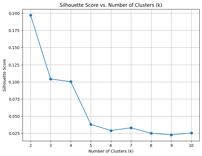
Silhouette scores against k
The best k values that we found were 4, 7, and 10.
- K-Means Clustering for Different k Values
Once we selected the best values of k based on the silhouette score, we applied K-means clustering with these values. We chose k = 4, 7, and 10 for analysis.
For each value of k:
We performed clustering and predicted the cluster labels for each data point. The resulting clusters were added as new columns to the dataframe (df), each corresponding to the cluster assignment. We visualized the clusters to understand how the data points were grouped in the reduced feature space (e.g., principal components). Visualization:
- If the data has two features (2D), we plotted a 2D scatter plot, coloring the points based on their cluster assignments. The centroids (cluster centers) were highlighted with red ‘x’ markers.
- If the data has three features (3D), we plotted the clusters in 3D space, again marking the centroids.
The market value of players was used as the primary feature for clustering, as it is a key indicator of player performance and value. The clustering results were analyzed to understand how players were grouped based on features and market value.
k = 4
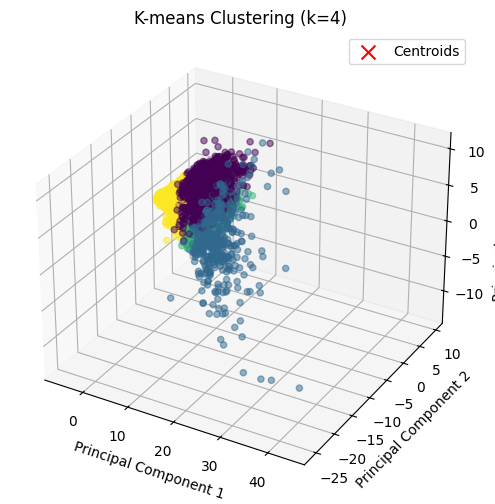
Clustering with k=4
k = 7
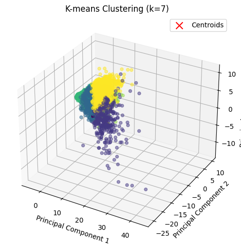
Clustering with k=7
k = 10
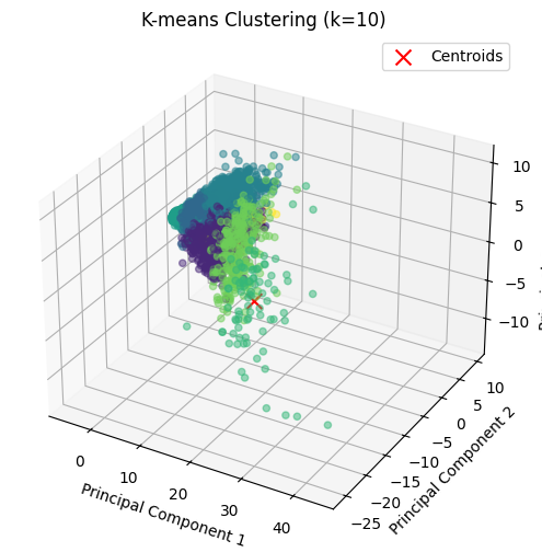
Clustering with k=7
- Market Value Analysis by Cluster
After clustering the data, we performed a market value analysis to understand how the clustering results might relate to specific characteristics of the data. We grouped the data by clusters and calculated various statistics for each cluster’s MarketValue, such as:
- Mean
- Median
- Standard deviation
- Count (number of points in each cluster)
- Min and Max values This analysis helped us identify the central tendencies of the Market Value for each cluster, providing insights into how the data points in each cluster compare to each other in terms of market value.
We then visualized this market value distribution using two types of plots:
- Box Plot: This shows the distribution of market values within each cluster, highlighting the median, quartiles, and potential outliers.
- Bar Plot (Mean): This shows the mean market value for each cluster.
The idea behind this analysis was to understand how the clustering algorithm grouped players based on their market value and whether there were any discernible patterns or trends in the data.
k = 4
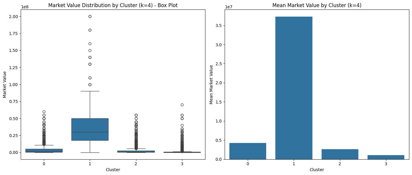
Box Plot of market value for each cluster (k = 4)
| Cluster | Mean | Median | Std Dev | Count | Min | Max |
|---|---|---|---|---|---|---|
| 0 | 4,258,093 | 1,500,000 | 6,863,090 | 2564 | 0 | 60,000,000 |
| 1 | 37,265,160 | 30,000,000 | 30,314,120 | 399 | 0 | 200,000,000 |
| 2 | 2,632,097 | 800,000 | 5,410,552 | 4148 | 0 | 55,000,000 |
| 3 | 1,027,634 | 225,000 | 3,293,389 | 5841 | 0 | 70,000,000 |
k = 7
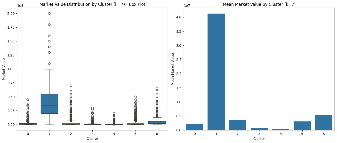
Box Plot of market value for each cluster (k = 7)
| Cluster | Mean | Median | Std Dev | Count | Min | Max |
|---|---|---|---|---|---|---|
| 0 | 2,286,096 | 600,000 | 5,247,828 | 748 | 0 | 45,000,000 |
| 1 | 41,257,990 | 35,000,000 | 32,001,260 | 319 | 0 | 200,000,000 |
| 2 | 3,590,506 | 850,000 | 7,355,122 | 2699 | 0 | 70,000,000 |
| 3 | 851,487 | 350,000 | 1,764,009 | 3010 | 0 | 30,000,000 |
| 4 | 498,181 | 125,000 | 1,490,811 | 2782 | 0 | 20,000,000 |
| 5 | 3,107,311 | 1,200,000 | 5,435,788 | 1759 | 0 | 50,000,000 |
| 6 | 5,339,541 | 2,200,000 | 7,777,065 | 1635 | 0 | 65,000,000 |
k = 10

Box Plot of market value for each cluster (k = 10)
| Cluster | Mean | Median | Std Dev | Count | Min | Max |
|---|---|---|---|---|---|---|
| 0 | 1,420,297 | 550,000 | 2,160,874 | 707 | 0 | 28,000,000 |
| 1 | 22,310,230 | 18,000,000 | 11,388,150 | 577 | 12,000,000 | 80,000,000 |
| 2 | 1,459,735 | 550,000 | 2,313,895 | 697 | 0 | 22,000,000 |
| 3 | 1,517,102 | 600,000 | 2,353,497 | 2,678 | 0 | 30,000,000 |
| 4 | 2,729,684 | 1,500,000 | 3,484,084 | 1,441 | 0 | 35,000,000 |
| 5 | 376,016 | 100,000 | 996,275 | 3,138 | 0 | 20,000,000 |
| 6 | 72,211,760 | 60,000,000 | 42,090,630 | 85 | 9,000,000 | 200,000,000 |
| 7 | 22,897,970 | 20,000,000 | 16,164,780 | 345 | 0 | 80,000,000 |
| 8 | 1,428,517 | 600,000 | 1,965,226 | 2,606 | 0 | 11,000,000 |
| 9 | 1,291,423 | 500,000 | 2,014,881 | 678 | 0 | 22,000,000 |
Hierarchical Clustering
Hierarchical clustering works by iteratively merging the closest data points into clusters, forming a tree structure (dendrogram). There are two main types:
- Agglomerative (Bottom-Up Approach): Each data point starts as its own cluster, and clusters merge step by step.
- Divisive (Top-Down Approach): The entire dataset starts as a single cluster, which then splits iteratively. In this analysis, we use the Agglomerative method with Ward’s linkage, which minimizes the variance within clusters.
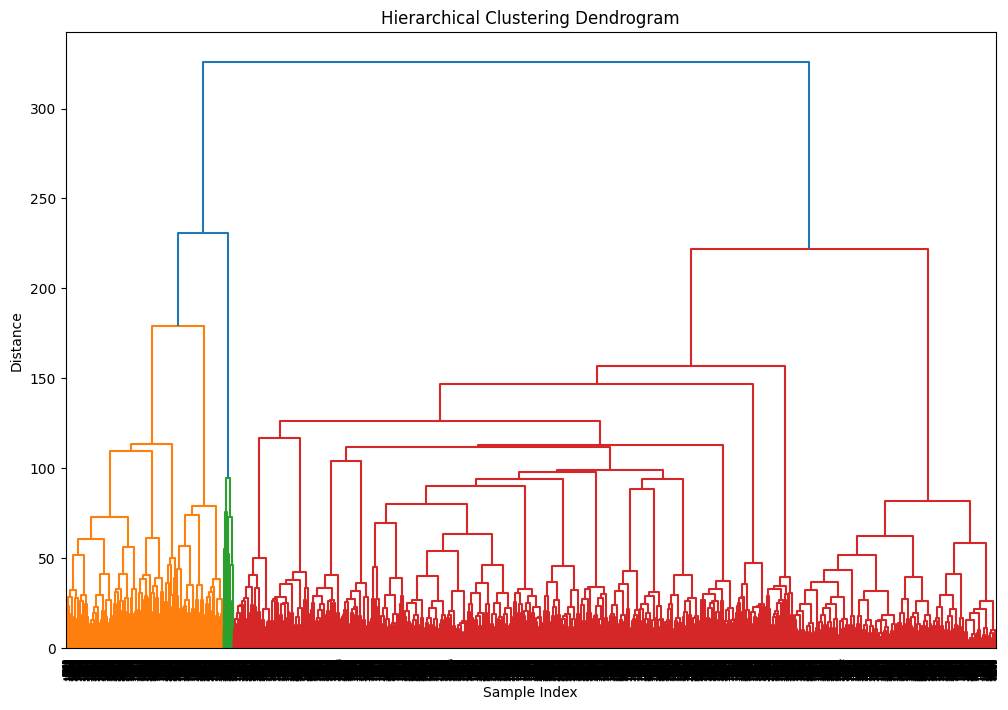
Hierarchichal Clustering Dendrogram
The dendrogram shows how the data points are merged into clusters based on their similarity. The height of the dendrogram represents the distance between clusters. By cutting the dendrogram at a certain height, we can determine the number of clusters.
From the dendrogram, we set the number of clusters to 100.
Market Value Analysis for Hierarchical Clustering (n_clusters=100)
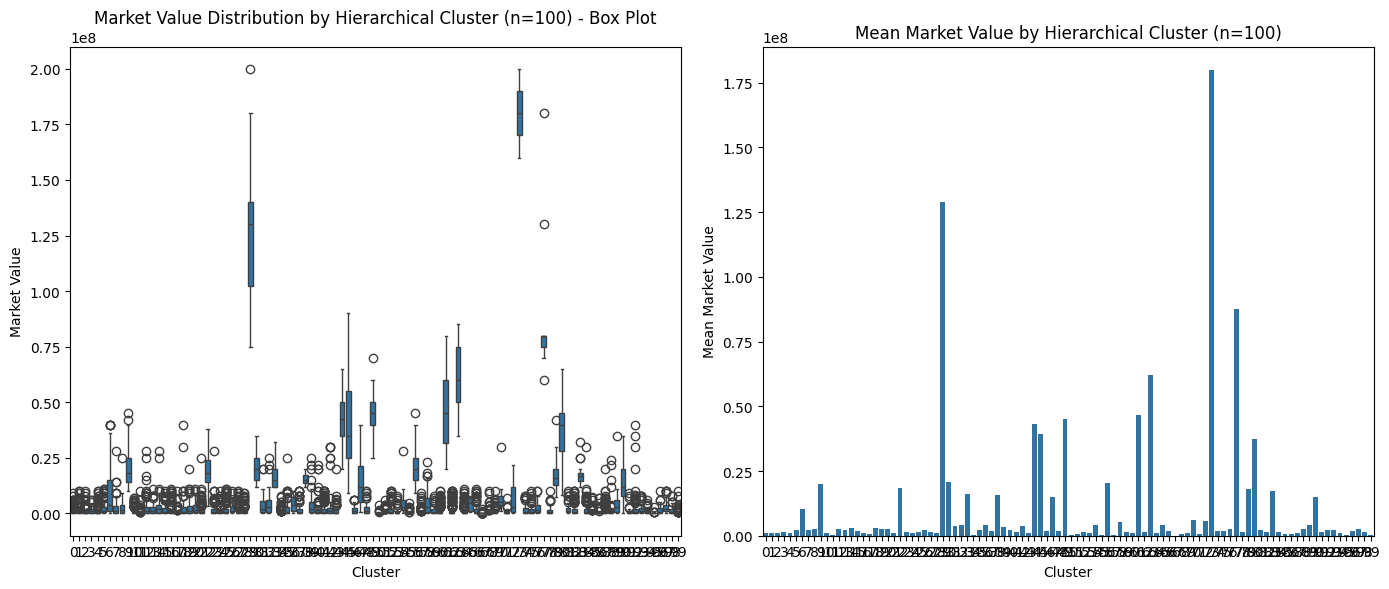
Box Plot of market value for each cluster (k = 100)
| Cluster | Mean | Median | Std Dev | Count | Min | Max |
|---|---|---|---|---|---|---|
| 0 | 1,083,373 | 500,000 | 1,459,915 | 249 | 0 | 9,000,000 |
| 1 | 1,036,769 | 450,000 | 1,567,847 | 294 | 0 | 10,000,000 |
| 2 | 869,588 | 400,000 | 1,308,720 | 243 | 0 | 10,000,000 |
| 3 | 1,583,673 | 1,000,000 | 1,624,860 | 49 | 75,000 | 6,000,000 |
| 4 | 983,457 | 400,000 | 1,540,844 | 337 | 0 | 10,000,000 |
| … | … | … | … | … | … | … |
| 95 | 214,361 | 100,000 | 461,706 | 47 | 0 | 3,000,000 |
| 96 | 1,667,935 | 850,000 | 2,022,881 | 46 | 0 | 10,000,000 |
| 97 | 2,730,469 | 2,000,000 | 2,636,836 | 64 | 100,000 | 10,000,000 |
| 98 | 1,516,406 | 800,000 | 1,759,522 | 64 | 50,000 | 8,000,000 |
| 99 | 381,682 | 150,000 | 894,933 | 315 | 0 | 10,000,000 |
[100 rows x 6 columns]
DBSCAN Clustering
We apply DBSCAN clustering to our dataset using Principal Component Analysis (PCA) transformed data for visualization. We set eps = 6 and min_samples = 3 as the hyperparameters for DBSCAN. The obtained clusters are visualized in 3D space. We get 9 clusters and 1465 noise points.
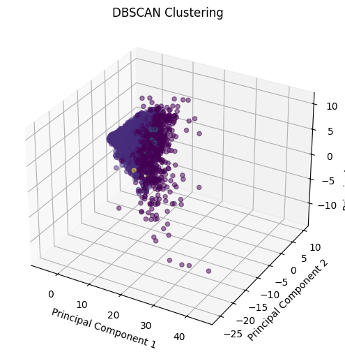
Clusters from DBScan
The market value distribution is as follows:
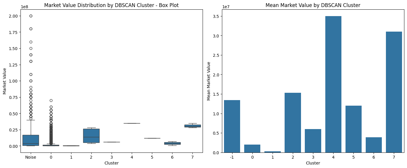
Box Plot of market value for each cluster (k = 9)
| Cluster | Mean | Median | Std Dev | Count | Min | Max |
|---|---|---|---|---|---|---|
| -1 | 13,423,280 | 4,000,000 | 22,190,480 | 1465 | 0 | 200,000,000 |
| 0 | 1,979,006 | 450,000 | 4,831,994 | 11463 | 0 | 70,000,000 |
| 1 | 300,000 | 400,000 | 264,575 | 3 | 0 | 500,000 |
| 2 | 15,333,333 | 13,500,000 | 11,893,980 | 6 | 4,000,000 | 28,000,000 |
| 3 | 6,000,000 | 6,000,000 | 0 | 3 | 6,000,000 | 6,000,000 |
| 4 | 35,000,000 | 35,000,000 | 0 | 3 | 35,000,000 | 35,000,000 |
| 5 | 12,000,000 | 12,000,000 | 0 | 3 | 12,000,000 | 12,000,000 |
| 6 | 3,850,000 | 4,000,000 | 3,227,615 | 3 | 550,000 | 7,000,000 |
| 7 | 31,000,000 | 30,000,000 | 3,605,551 | 3 | 28,000,000 | 35,000,000 |
Comparison of Clustering Results
Ideally, we would like to explore more clustering using clustering methods in order to identify underrated and overrated players. We can observe that hierarchichal clustering was able to generate a lot of clusters thus providing more granularity in the data. DBSCAN was able to identify noise points and cluster the data accordingly. K-means clustering was able to group the data into a specified number of clusters.
A potential limitation is for the players in the defender postions who are not able to score goals. This might lead to a confusion when clustering and checking for players with similar market value potential. But the core idea of checking market value is to identify players with similar potential with lower market value which can be helpful for scouting.
The code for implementing clustering can be found here