Football Analytics - Model Implementation - Decision Trees

Overview of Decision Trees

A Decision Tree is a versatile, supervised machine learning algorithm employed for both classification and regression tasks. It structures data into a tree-like model of decisions and their possible consequences, facilitating straightforward interpretation and decision-making.​

Structure of a Decision Tree:

• Root Node: Represents the entire dataset and initiates the splitting process.​
• Internal Nodes (Decision Nodes): Each node denotes a test or decision on an attribute, leading to further branches.​
• Branches: Illustrate the outcomes of tests, directing to subsequent nodes.​
• Leaf Nodes (Terminal Nodes): Indicate the final decision or prediction outcome.​

Applications of Decision Trees:

• Classification Tasks: Assigning data points to predefined categories, such as determining if an email is spam or not.​
• Regression Tasks: Predicting continuous values, like forecasting housing prices based on various features.​

​Decision Trees are versatile models capable of handling various types of input features during training. These features can be broadly categorized into:​

1. Numerical Features:
   • Continuous Variables: These are features that can take on any value within a range. Examples include age, income, temperature, or height. Decision Trees can effectively process continuous data by determining optimal split points that minimize impurity measures like Gini Impurity or Entropy.​
2. Categorical Features:
   • Nominal Variables: These represent categories without any inherent order, such as colors (red, blue, green) or types of animals (cat, dog, bird). Decision Trees handle nominal data by creating branches for each category, partitioning the data accordingly.​
   • Ordinal Variables: These categories have a meaningful order but no fixed interval between them, like education levels (high school, bachelor’s, master’s). Decision Trees can exploit the order in ordinal data to make more informed splits.​

One of the strengths of Decision Trees is their ability to manage datasets with a mix of numerical and categorical features without requiring extensive preprocessing. This flexibility simplifies the data preparation process and allows for the natural handling of diverse data types within a single model.​

Example of a Decision Tree:

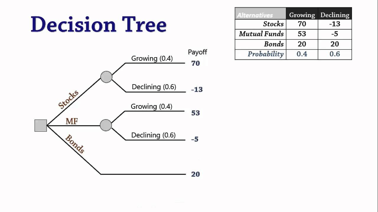
Decision Tree

Training a Decision Tree:

The construction of a decision tree involves recursively partitioning the dataset into subsets based on attribute values, aiming to increase the homogeneity of the resulting groups. This process continues until a stopping criterion is met, such as achieving a minimum number of samples in a node or reaching a maximum tree depth.​

Splitting Criteria

To determine the optimal way to split nodes, decision trees utilize measures like Gini Impurity, Entropy, and Information Gain.​

• Entropy: Measures the disorder or impurity in a dataset. A dataset with only one class has an entropy of zero, indicating perfect purity.​

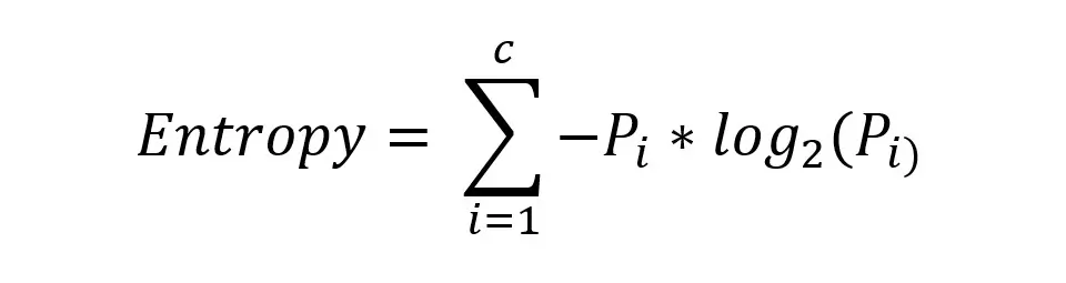
Formula for entropy

Where p_i is the proportion of samples in class i, and c is the total number of classes.

• Information Gain: Quantifies the reduction in entropy after a dataset is split on an attribute. Higher information gain indicates a more effective split.​

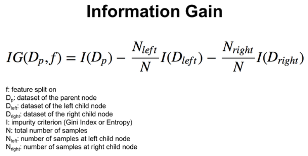
Formula for information gain

• Gini Impurity: Measures the likelihood of misclassifying a randomly chosen element from the dataset. A lower Gini Impurity indicates a more homogeneous group.​

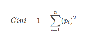
Formula for Gini impurity

Where p_i is the proportion of samples in class i, and c is the total number of classes.

Dataset Preparation

The general dataset used here has numerical and categorical vatiables. The target variable is the MarketValue that is binned into 3 classes that:

• 0: Less valuable player
• 1: Moderately valuable player
• 2: Highly valuable player

The original dataset:

Parent Dataset

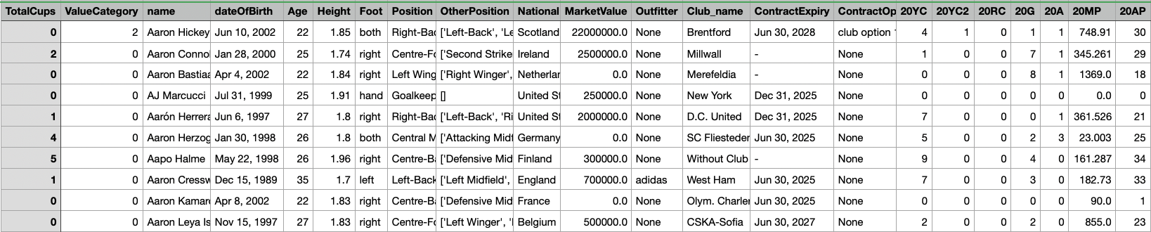
Link to dataset

Decision Trees Dataset

The dataset comprises detailed football player attributes, categorized into two types:

Categorical Features:

• Foot: Preferred foot of the player (left/right)
• Position: Primary playing position (e.g., forward, midfielder, defender, goalkeeper)
• OtherPosition: Alternative positions the player can play
• National: Nationality of the player
• Club_name: Current club the player represents
• ContractOption: Contract details such as buyout clauses and renewal options
• Outfitter: Brand sponsoring the player’s gear (e.g., Nike, Adidas, Puma)

Numerical Features:

• Age
• Yellow and Red Cards (YC, RC) for different seasons
• Goals (G) and Assists (A)
• Matches Played (MP) and Appearances (AP)
• Total Cups Won

Target Variable:

• ValueCategory: This variable represents different market value categories for players, enabling classification-based modeling to predict a player’s value segment.

Data Preprocessing and Train-Test Split

• Label Encoding of Categorical Features: Machine learning models require numerical input. To address this, categorical variables such as ‘Position’ and ‘Club_name’ are transformed into numerical values using Label Encoding. Each unique category is assigned an integer value, preserving meaningful distinctions while making the data model-ready.

• Class Balancing Through Resampling: Market value distribution is often imbalanced, with more players in mid-value ranges and fewer in extreme categories. To ensure a well-balanced dataset for training, we apply resampling techniques, either upsampling minority classes or downsampling majority classes. This creates an even distribution across market value categories, helping the model generalize better across different player valuations.

• Train-Test Split: The dataset is split into 80% training and 20% testing, ensuring the model learns from a diverse set of data while being evaluated on unseen examples.

• Feature Scaling for Numerical Columns: Performance metrics like goals scored or matches played vary significantly in magnitude. To normalize these differences, Standard Scaling (Z-score normalization) is applied, ensuring that all numerical features have a mean of 0 and a standard deviation of 1. This prevents certain features from disproportionately influencing the model.

Screenshots and Links to Datasets

X-train

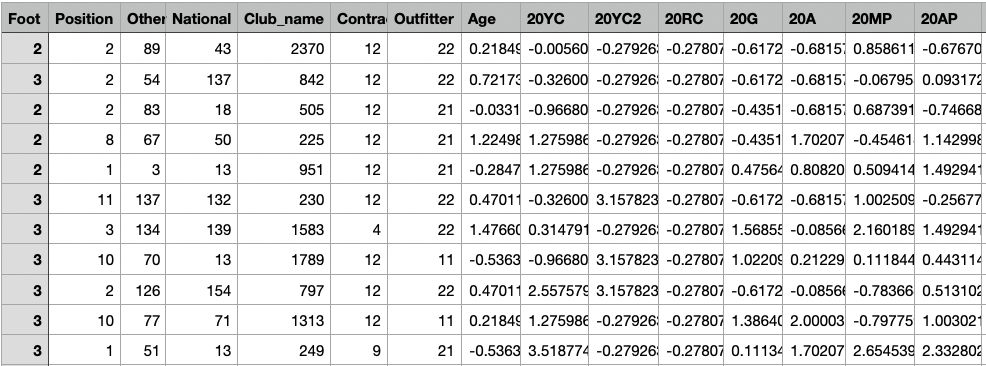
X-train for Decision Tree Model

The shape of X-train is (2400, 51). Link to dataset

X-test

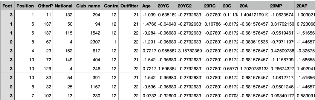
X-test for Decision Tree Model

The shape of X-test is (600, 51). Link to dataset

y-train

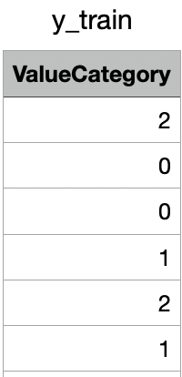
y-train for Decision Tree Model

The shape of y-train is (2400,). Link to dataset

y-test

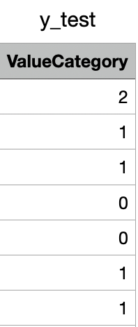
y-test for Decision Tree Model

The shape of y-test is (600,). Link to dataset

Code files

The code used for dataset preparation and training the Decision Tree model is available here

Results

Decision Tree Model 1 (Max Depth 3)

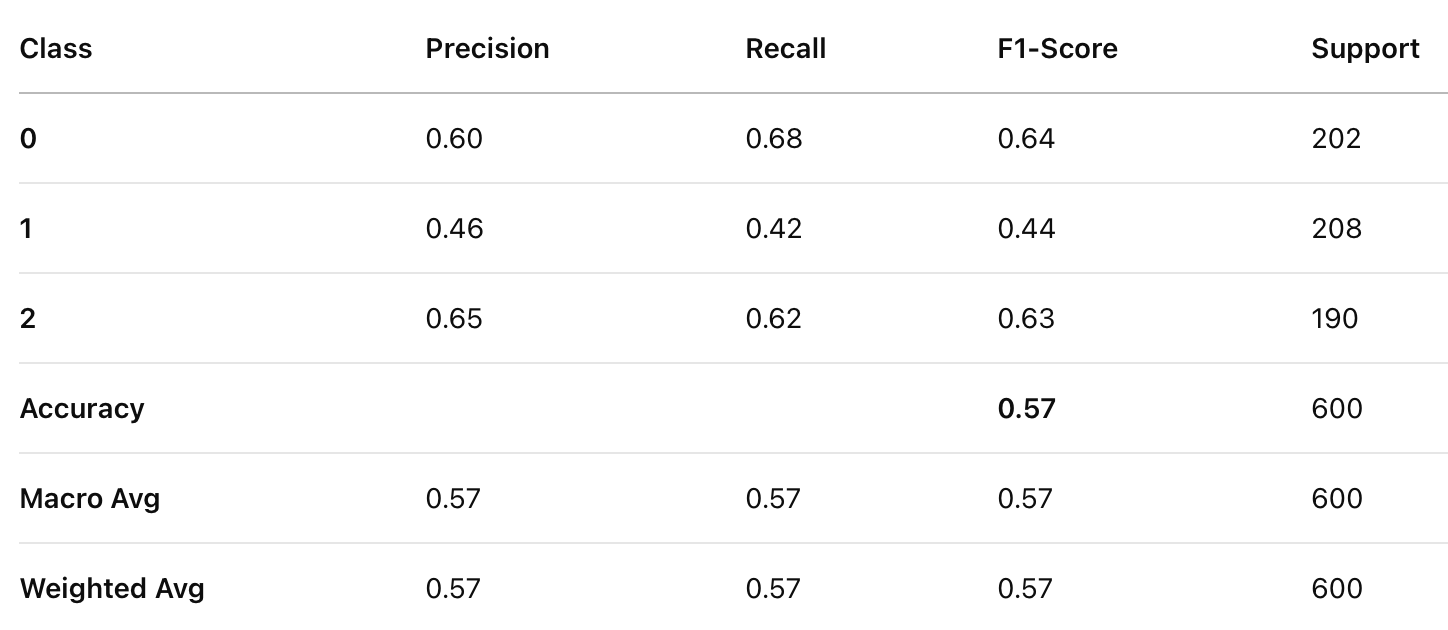
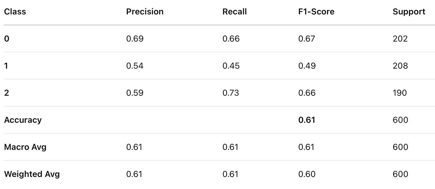
Classification Report for Decision Tree Model 1

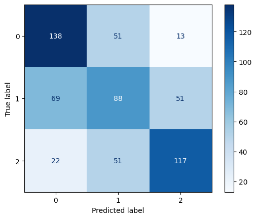
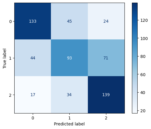
Confusion Matrix for Decision Tree Model 1

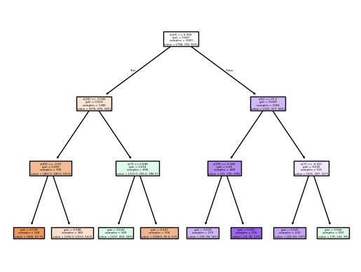
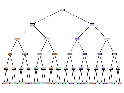
Decision Tree Model 1 Vizualization

Decision Tree Model 2 (Max Depth 5)

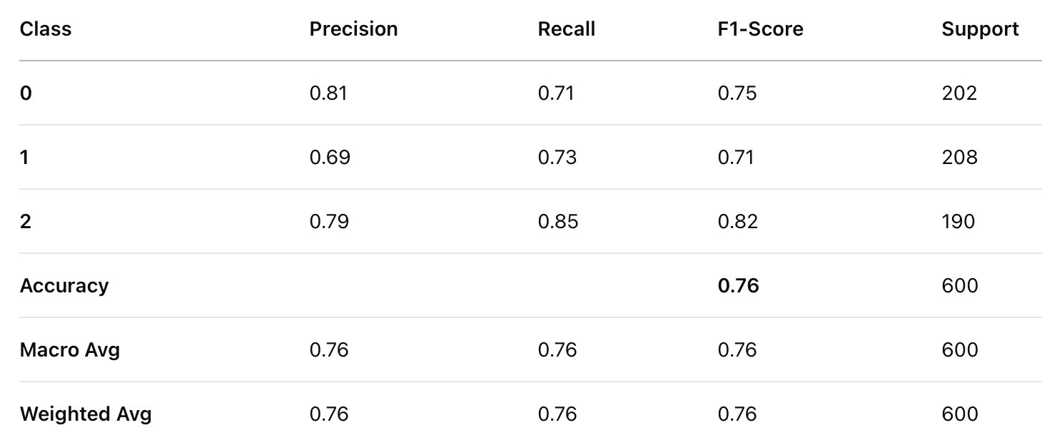
Classification Report for Decision Tree Model 2

Confusion Matrix for Decision Tree Model 2

Decision Tree Model 2 Vizualization

Decision Tree Model 2 (No Max Depth)

Classification Report for Decision Tree Model 3

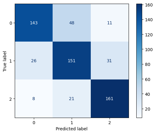
Confusion Matrix for Decision Tree Model 3

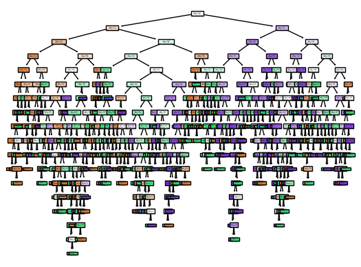
Decision Tree Model 3 Vizualization

Comparison of Decision Tree Models

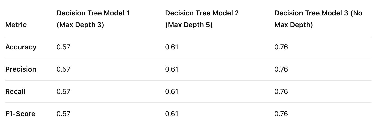
Comparison of all three DT models

The accuracy, precision, recall, and F1-score improved as the depth of the decision tree increased. A deeper decision tree (no max depth) performed significantly better than shallower trees, suggesting that capturing deeper patterns in player attributes is crucial for valuation prediction.

Conclusion

Metrics like goals, assists, and matches played are strong indicators of a player’s market value. Players with higher contributions in these areas are more likely to belong to higher value categories. Certain positions (e.g., forwards and attacking midfielders) tend to have higher valuations, possibly due to their direct impact on scoring. Players from prestigious clubs and footballing nations often hold higher market values, reflecting real-world trends in transfer market dynamics.

Overall, the results confirm that player market value is influenced by a mix of performance metrics, positional roles, and external factors like club reputation, and increasing model complexity can significantly enhance predictive accuracy.

Back to Home