Football Analytics - Model Implementation - Ensemble Methods

Overview

Ensemble methods are techniques that combine multiple models to improve overall prediction performance compared to using a single model. These methods help reduce overfitting, increase accuracy, and make models more robust. The main idea is that multiple weak learners (individual models) can be combined to form a strong learner.

There are two main types of ensemble methods:

• Bagging (Bootstrap Aggregating) – Multiple models are trained independently using different random subsets of the data, and their predictions are averaged (or majority voted). Example: Random Forests.
• Boosting – Models are trained sequentially, where each model corrects the errors of the previous one. Example: Gradient Boosting, XGBoost.

Random Forest

Random Forest is an ensemble learning technique that extends decision trees by using bagging (Bootstrap Aggregation). It creates multiple decision trees and combines their predictions (by averaging in regression or voting in classification).

How It Works:

A dataset is randomly sampled with replacement (bootstrap sampling). Multiple decision trees are trained on different subsets of the data. Each tree predicts an outcome, and the final prediction is made by averaging (regression) or majority voting (classification). It also uses feature randomness, selecting only a subset of features for each tree, reducing overfitting.

Advantages:

• Reduces overfitting (compared to a single decision tree).
• Works well with high-dimensional data.
• Handles missing values well.

Disadvantages:

• Slower compared to single decision trees.
• Not as good for very large datasets where computation time is crucial.

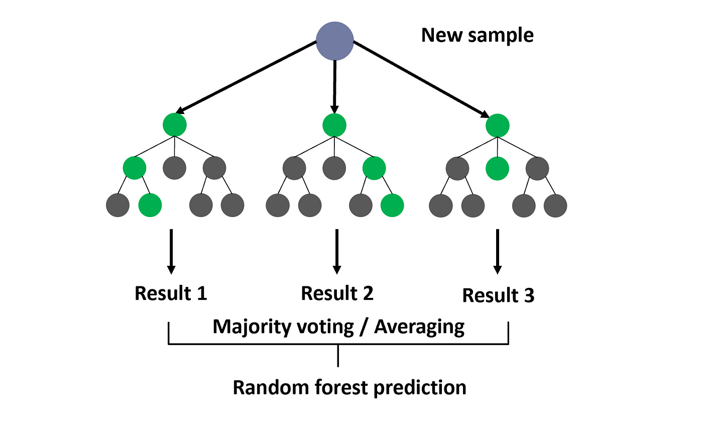
Visual Respresentation of Random Forests

Gradient Boosting

Gradient Boosting is an advanced boosting technique that builds models sequentially, where each new model corrects the errors of the previous ones. It minimizes a loss function using gradient descent.

How It Works:

A weak model (often a decision tree) is trained on the data. Errors from this model are calculated, and a new model is trained to correct these errors. This process repeats, with each new model focusing more on difficult-to-predict cases. The final model is a weighted sum of all weak models.

Advantages:

• More accurate than Random Forest for some structured datasets.
• Works well with smaller datasets and complex relationships.

Disadvantages:

• More prone to overfitting if not carefully tuned.
• Computationally expensive and slower than Random Forest.

XGBoost

XGBoost is an optimized version of Gradient Boosting that is faster, more efficient, and handles missing values better.

Key Improvements Over Standard Gradient Boosting:

• Uses regularization (L1 & L2) to reduce overfitting.
• Uses parallelization for faster training.
• Implements shrinkage (learning rate) to slow down updates and improve generalization.
• Uses weighted quantile sketching to handle imbalanced datasets effectively.

Advantages:

• Faster than traditional Gradient Boosting.
• More scalable and efficient, works well with large datasets.
• Better handling of missing values and feature interactions.

Disadvantages:

• More complex and harder to tune than Random Forest.
• Needs careful hyperparameter tuning for best performance.

Dataset Preparation

The dataset used here is the same as the one used for decision trees.

The general dataset used here has numerical and categorical vatiables. The target variable is the MarketValue that is binned into 3 classes that:

• 0: Less valuable player
• 1: Moderately valuable player
• 2: Highly valuable player

The original dataset:

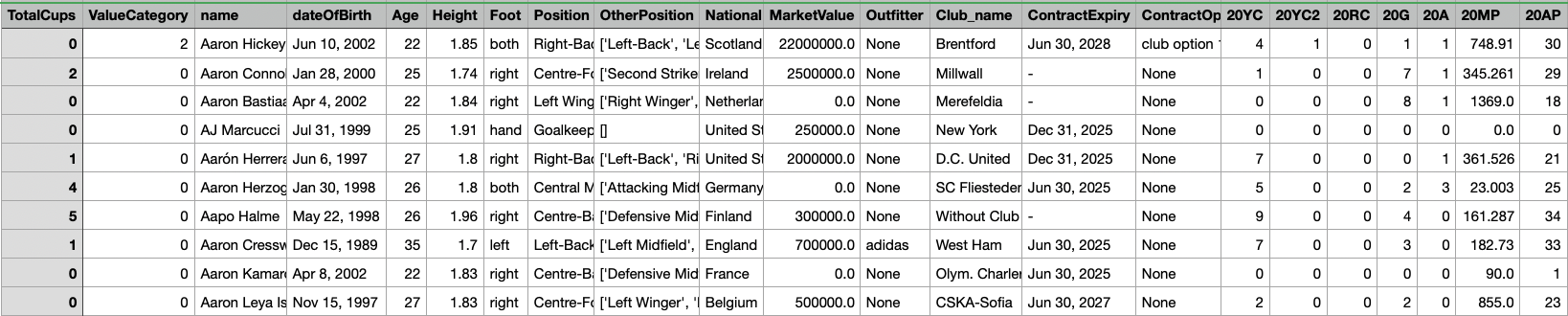
Parent Dataset

Link to dataset

Dataset Info

The dataset comprises detailed football player attributes, categorized into two types:

Categorical Features:

• Foot: Preferred foot of the player (left/right)
• Position: Primary playing position (e.g., forward, midfielder, defender, goalkeeper)
• OtherPosition: Alternative positions the player can play
• National: Nationality of the player
• Club_name: Current club the player represents
• ContractOption: Contract details such as buyout clauses and renewal options
• Outfitter: Brand sponsoring the player’s gear (e.g., Nike, Adidas, Puma)

Numerical Features:

The dataset includes various performance metrics collected over multiple seasons, such as:

• Age
• Yellow and Red Cards (YC, RC) for different seasons
• Goals (G) and Assists (A)
• Matches Played (MP) and Appearances (AP)
• Total Cups Won

Target Variable:

• ValueCategory: This variable represents different market value categories for players, enabling classification-based modeling to predict a player’s value segment.

Data Preprocessing and Train-Test Split

• Label Encoding of Categorical Features: Machine learning models require numerical input. To address this, categorical variables such as ‘Position’ and ‘Club_name’ are transformed into numerical values using Label Encoding. Each unique category is assigned an integer value, preserving meaningful distinctions while making the data model-ready.

• Class Balancing Through Resampling: Market value distribution is often imbalanced, with more players in mid-value ranges and fewer in extreme categories. To ensure a well-balanced dataset for training, we apply resampling techniques, either upsampling minority classes or downsampling majority classes. This creates an even distribution across market value categories, helping the model generalize better across different player valuations.

• Train-Test Split: The dataset is split into 80% training and 20% testing, ensuring the model learns from a diverse set of data while being evaluated on unseen examples.

• Feature Scaling for Numerical Columns: Performance metrics like goals scored or matches played vary significantly in magnitude. To normalize these differences, Standard Scaling is applied, ensuring that all numerical features have a mean of 0 and a standard deviation of 1. This prevents certain features from disproportionately influencing the model.

Screenshots and Links to Datasets

X-train

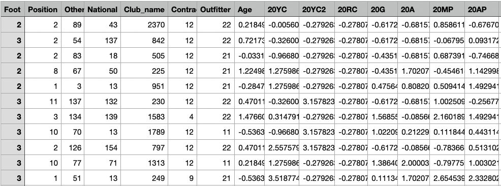
X-train for Decision Tree Model

The shape of X-train is (2400, 51). Link to dataset

X-test

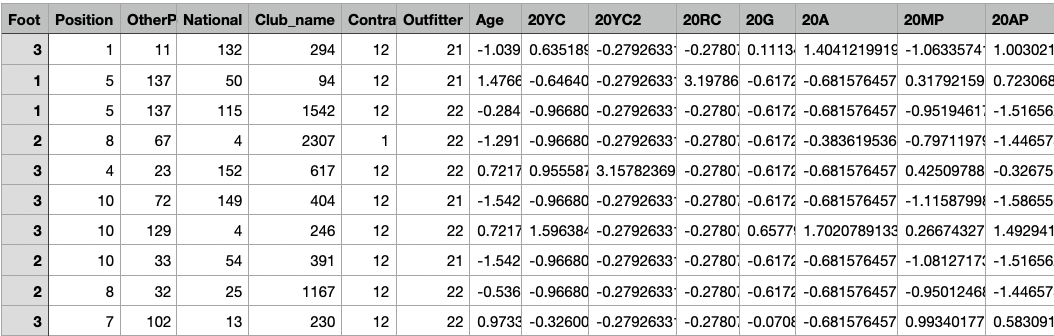
X-test for Decision Tree Model

The shape of X-test is (600, 51). Link to dataset

y-train

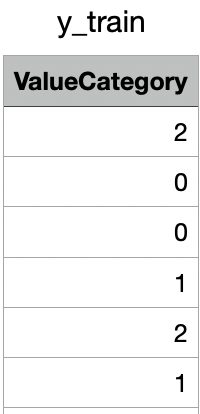
y-train for Decision Tree Model

The shape of y-train is (2400,). Link to dataset

y-test

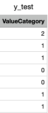
y-test for Decision Tree Model

The shape of y-test is (600,). Link to dataset

Code files

The code used for dataset preparation and training the Decision Tree model is available here

Results

Random Forest

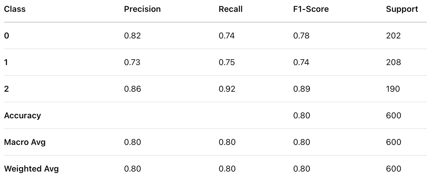
Classification Report for Random Forest Classifier

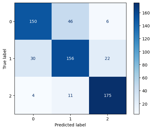
Confusion Matrix for Random Forest Classifier

Gradient Boosting

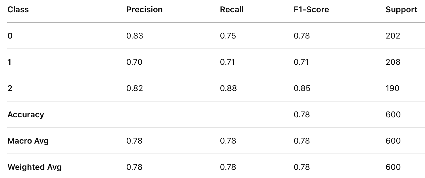
Classification Report for Gradient Boosting Classifier

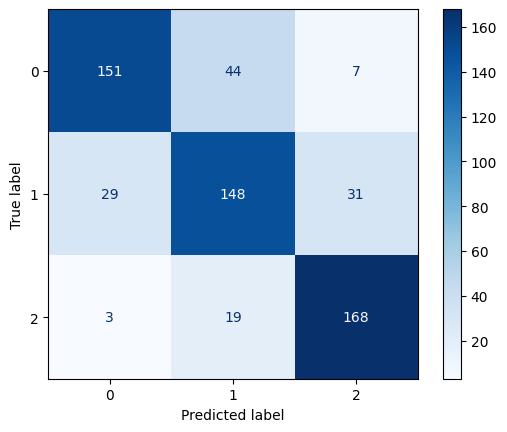
Confusion Matrix for Gradient Boosting Classifier

XGBoost

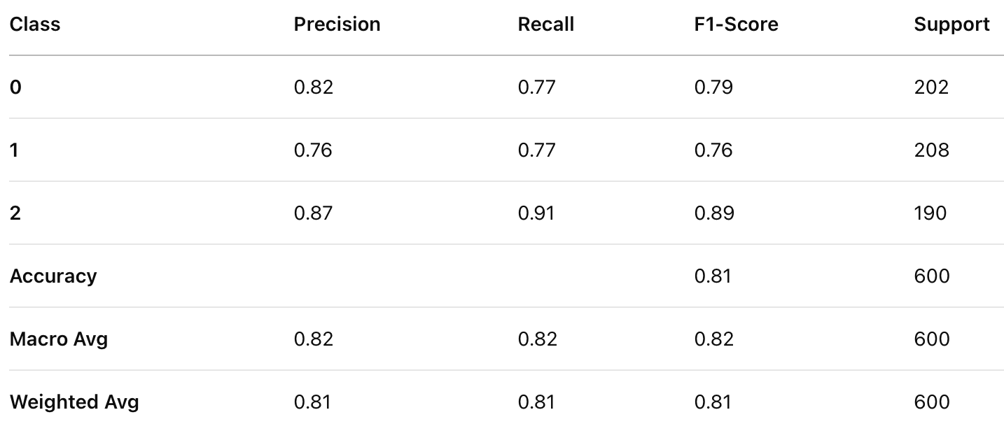
Classification Report for XGBoost Classifier

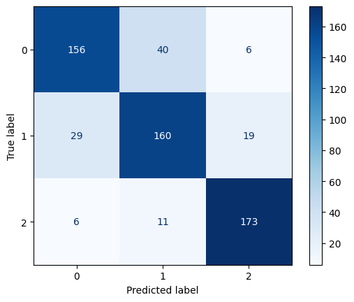
Confusion Matrix for XGBoost Classifier

Comparison

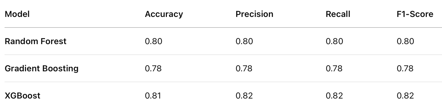
Comparison of Classifiers

XGBoost achieved the highest accuracy (0.81), followed by Random Forest (0.80), and Gradient Boosting performed the lowest (0.78). XGBoost outperformed the other models in both precision and recall, indicating better balance in handling false positives and false negatives. XGBoost also achieved the highest F1-score (0.82), making it the most reliable model in terms of balanced performance.

While Random Forest performed slightly better than Gradient Boosting, its performance was still lower than XGBoost across all metrics.Gradient Boosting had the lowest performance among the three models, suggesting it might not generalize as well for this dataset.

Conclusion

Based on the evaluation, XGBoost is the best-performing model for this classification task, achieving the highest accuracy, precision, recall, and F1-score. While Random Forest also performed well, XGBoost’s superior results make it the preferable choice. Gradient Boosting, while still effective, underperformed relative to the other models and might need further tuning to improve results.

Back to Home