
Football Analytics - Model Implementation - Naive Bayes
Overview of Naïve Bayes
Naïve Bayes (NB) classifiers are a family of probabilistic algorithms based on Bayes’ Theorem, which predict the category of a sample by assuming that the presence of a particular feature is independent of the presence of any other feature, given the class label. Despite this “naïve” independence assumption, NB classifiers have proven effective, especially in high-dimensional datasets.
Applications of Naïve Bayes
Here are some key areas where Naïve Bayes algorithms excel:
- Text Classification
- Medical Diagnosis
- Recommendation Systems
Each of these applications leverages the algorithm’s ability to handle large feature sets while maintaining computational efficiency.
Types of Naïve Bayes Classifiers:
-
Multinomial Naïve Bayes Assumes that features represent frequencies of events, such as word counts in text classification. It models the distribution of each feature as multinomial. Ideal for text classification tasks where the data is represented as word frequency vectors.
-
Gaussian Naïve Bayes Assumes that features follow a Gaussian (normal) distribution. It is suitable for continuous data and is often used in scenarios where the features are real-valued. Suitable for datasets with continuous numerical features that are approximately normally distributed.
-
Bernoulli Naïve Bayes Designed for binary/boolean features, indicating the presence or absence of a feature. It models each feature as a binary variable. Commonly used in text classification with binary term occurrence features (e.g., whether a word appears in a document or not).
-
Categorical Naïve Bayes Handles categorical data where features can take on a limited set of discrete values without any order. It models each feature’s distribution as categorical. Applicable when dealing with categorical features that are not ordinal, such as color, brand, or type categories.
Comparison
The Categorical Naive Bayes (CNB), Multinomial Naive Bayes (MNB), and Gaussian Naive Bayes (GNB) models must be disjoint because they handle fundamentally different types of data and require distinct preprocessing techniques:
Feature Types:
- CNB is designed for categorical data, where features represent discrete categories (e.g., “Left” or “Right” for foot preference).
- MNB is designed for numerical count-based data, where features represent frequencies or counts (e.g., word counts in text classification).
- GNB is designed for continuous data, where features are assumed to follow a Gaussian/normal distribution (e.g., height, weight, or other measured values).
Encoding & Interpretation:
- CNB relies on Label Encoding, which maps categorical values to integers but still treats them as distinct categories.
- MNB expects raw numeric values (such as word frequencies) and assumes they follow a multinomial distribution.
- GNB works with continuous values and assumes each feature follows a normal distribution with class-specific mean and variance.
Probability Assumptions:
- CNB calculates probabilities based on categorical frequencies.
- MNB computes probabilities assuming the numeric features represent counts or frequencies.
- GNB models the likelihood of each feature using Gaussian probability density functions.
Since each model is tailored to a specific type of input with different underlying probability distributions, mixing them would distort the mathematical assumptions underlying their probability computations. Hence, they must remain disjoint—each trained on its respective subset of features appropriate to its distributional assumptions.
Why Smoothing is Required for NB Models
Smoothing techniques, such as Laplace smoothing, are employed to handle the issue of zero probabilities in NB models. When a particular feature-class combination is absent in the training data, it results in a probability of zero, which can nullify the entire probability calculation for a sample. Smoothing adds a small value to all probability estimates, ensuring that no probability is ever exactly zero, thereby improving the model’s robustness.
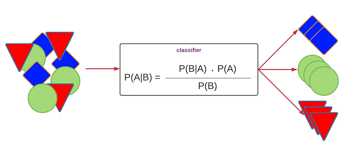
Visual representation of working of NB Classifiers
Naïve Bayes classifiers are grounded in Bayes’ Theorem, a fundamental principle in probability theory that describes how to update the probability of a hypothesis as more evidence becomes available. This simplification allows for efficient computation, especially in high-dimensional spaces, making Naïve Bayes classifiers particularly effective for tasks like text classification. By applying Bayes’ Theorem with the independence assumption, Naïve Bayes classifiers calculate the posterior probability for each class and assign the sample to the class with the highest posterior probability. Despite the strong independence assumption, these classifiers often perform well in practice, even when the independence condition is not strictly met.
Dataset Preparation
The general dataset used here has numerical and categorical vatiables. The target variable is the MarketValue that is binned into 3 classes that:
- 0: Less valuable player
- 1: Moderately valuable player
- 2: Highly valuable player
The original dataset:
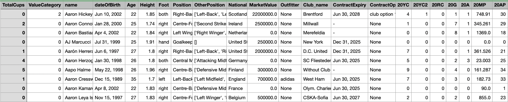
Parent Dataset
Categorical Naïve Bayes Dataset
The dataset consists of football player attributes, including categorical features such as:
- Foot (preferred foot of the player)
- Position (primary playing position)
- OtherPosition (alternative positions the player can play)
- National (nationality of the player)
- Club_name (current club)
- ContractOption (contract details like buyout clauses)
- Outfitter (brand sponsoring the player’s gear)
The target variable, ValueCategory, represents different categories of market value for a player. This dataset provides an opportunity to understand how categorical factors contribute to determining a player’s worth.
Data Preprocessing and Train-Test Split
Before training the model, preprocessing steps are:
-
Label Encoding: Since machine learning models work with numerical data, categorical columns are encoded using Label Encoding, converting each unique category into a numerical representation.
-
Class Balancing: The dataset is likely to have an imbalance in player value categories, meaning some categories may have significantly fewer samples than others. To address this, we perform resampling to ensure each class has an equal number of samples.
-
Train-Test Split: The dataset is split into 80% training and 20% testing, ensuring the model learns from a diverse set of data while being evaluated on unseen examples.
-
Outlier Handling: To prevent test data from having values not seen in training, any test set values exceeding the maximum training value in a particular feature are capped.
Screenshots and Links to Datasets
X-train
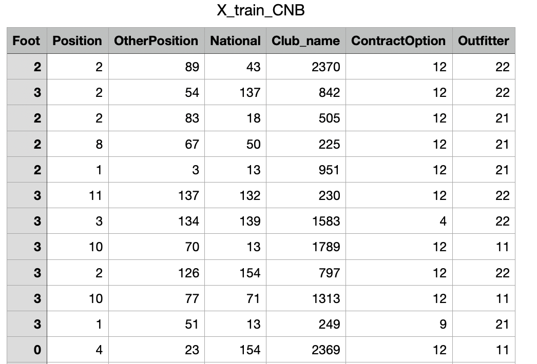
X-train for CNB
The shape of X-train is (2400, 7). Link to dataset
X-test
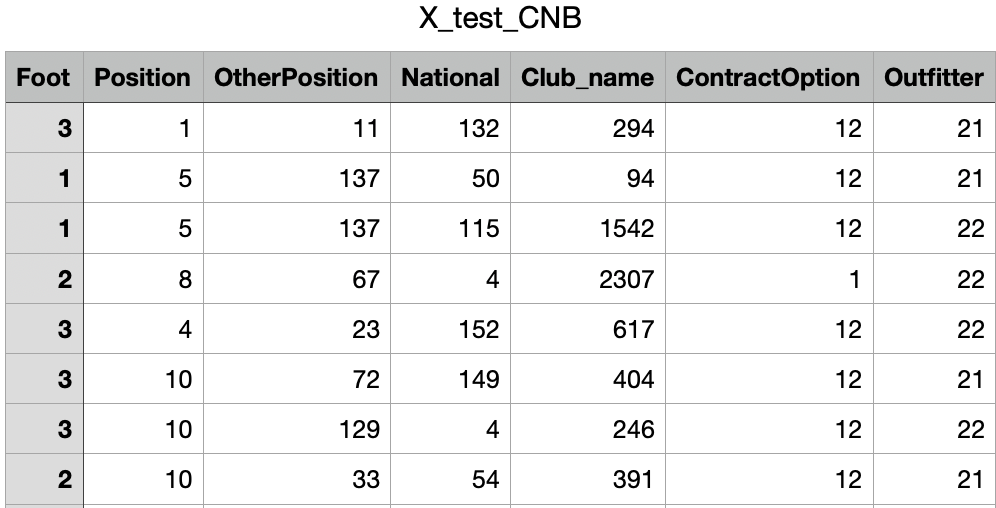
X-test for CNB
The shape of X-test is (600, 7). Link to dataset
y-train
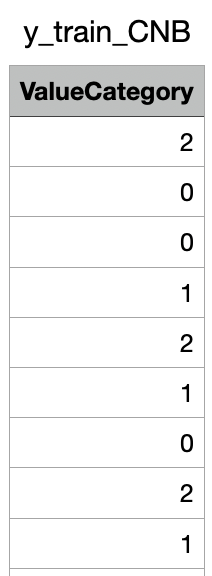
The shape of y-train is (2400,). Link to dataset
y-test
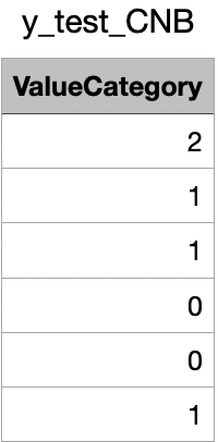
y-test for CNB
The shape of y-test is (600,). Link to dataset
Multinomial Naïve Bayes Dataset
The dataset consists of football player attributes, including categorical and numerical features. These features help analyze how different factors influence a player’s market value.
Numerical Features:
- Performance Metrics Across Seasons: Includes appearances (MP), goals (G), assists (A), yellow cards (YC), red cards (RC), and other relevant statistics.
Target Variable:
- ValueCategory: Represents different categories of market value for a player, classifying them into three groups (0, 1, or 2).
Data Preprocessing and Train-Test Split
Before training the model, several preprocessing steps are applied to ensure data quality and improve model performance:
-
Class Balancing: The dataset may have an imbalance in player value categories, meaning some categories may have significantly fewer samples than others. To address this, we perform resampling to ensure each class has an equal number of samples (1,000 per category).
-
Train-Test Split: The dataset is split into 80% training and 20% testing, ensuring that the model learns from a diverse set of data while being evaluated on unseen examples.
-
Outlier Handling: To prevent the model from encountering values in the test set that were not seen during training, any test set values exceeding the maximum observed training values in a particular feature are capped.
Screenshots and Links to Datasets
X-train
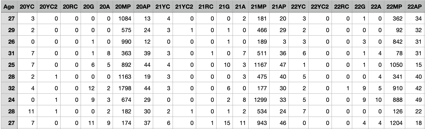
X-train for MNB
The shape of X-train is (2400, 44). Link to dataset
X-test
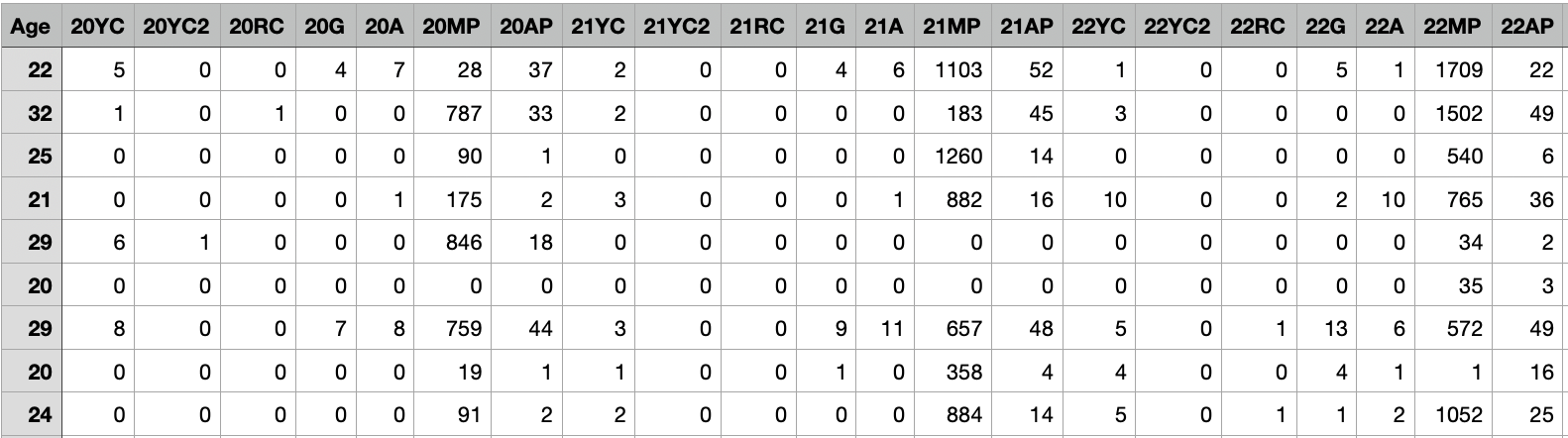
X-test for MNB
The shape of X-test is (600, 44). Link to dataset
y-train
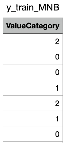
y-train for MNB
The shape of y-train is (2400,). Link to dataset
y-test
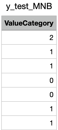
y-test for MNB
The shape of y-test is (600,). Link to dataset
Gaussian Naïve Bayes Dataset
The dataset consists of football player attributes, both categorical and numerical, which are used to analyze factors influencing a player’s market value. The goal is to predict the player’s value category using machine learning.
Numerical Features:
- Age: Player’s age.
- Performance Metrics (2020-2025): Includes goals (G), assists (A), match appearances (MP), yellow cards (YC), red cards (RC), and other statistics across different seasons.
- TotalCups: Number of tournaments the player has participated in.
Target Variable:
- ValueCategory: Categorizes players into three groups (0, 1, or 2) based on their market value.
Data Preprocessing and Train-Test Split
Before training the model, various preprocessing steps were applied to enhance data quality and improve model performance.
-
Class Balancing: Since the dataset may have an imbalance in player value categories, resampling was performed to ensure each category contained an equal number of samples (1,000 per class).
-
Train-Test Split: The dataset was divided into 80% training and 20% testing to enable model learning on diverse data while being evaluated on unseen examples.
-
Feature Scaling: Standardization was applied to numerical features to ensure uniformity, as Naïve Bayes models rely on feature distributions.
Screenshots and Links to Datasets
X-train
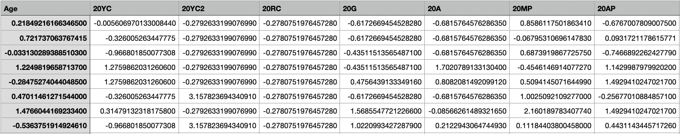
X-train for GNB
The shape of X-train is (2400, 44). Link to dataset
X-test
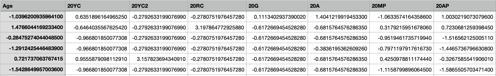
X-test for GNB
The shape of X-test is (600, 44). Link to dataset
y-train
The shape of y-train is (2400,). Link to dataset
y-test
y-test for GNB
The shape of y-test is (600,). Link to dataset
Code files
These files are used for the dataset preparation and model training.
Results
Categorical Naïve Bayes
Classification Report for CNB
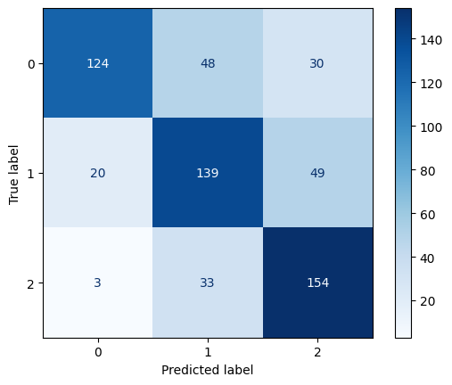
Confusion Matrix for CNB
Multinomial Naïve Bayes
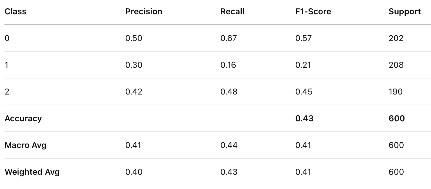
Classification Report for MNB
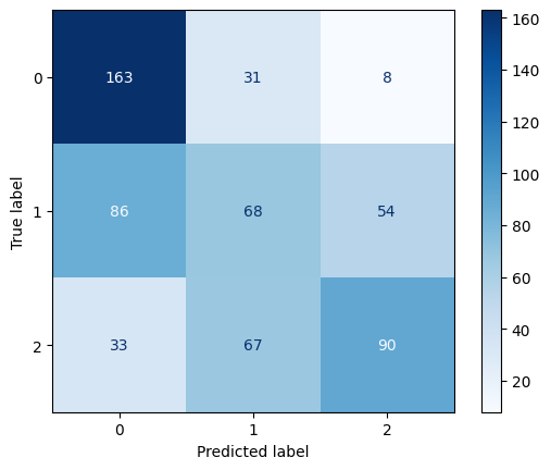
Confusion Matrix for MNB
Gaussian Naïve Bayes
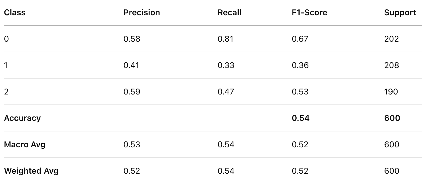
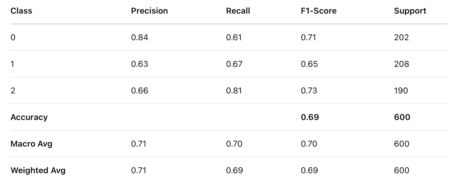
Classification Report for GNB
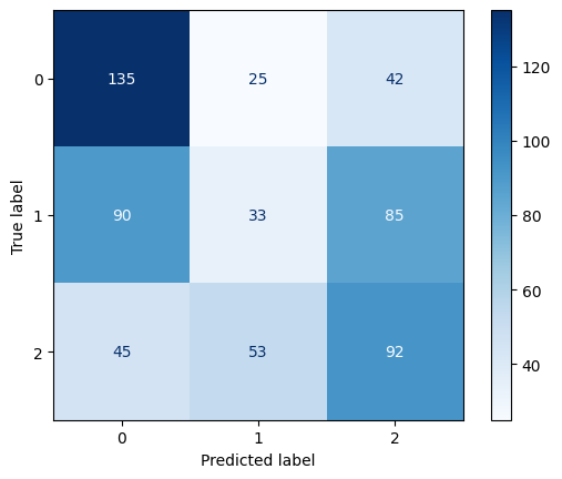
Confusion Matrix for GNB
Comparison
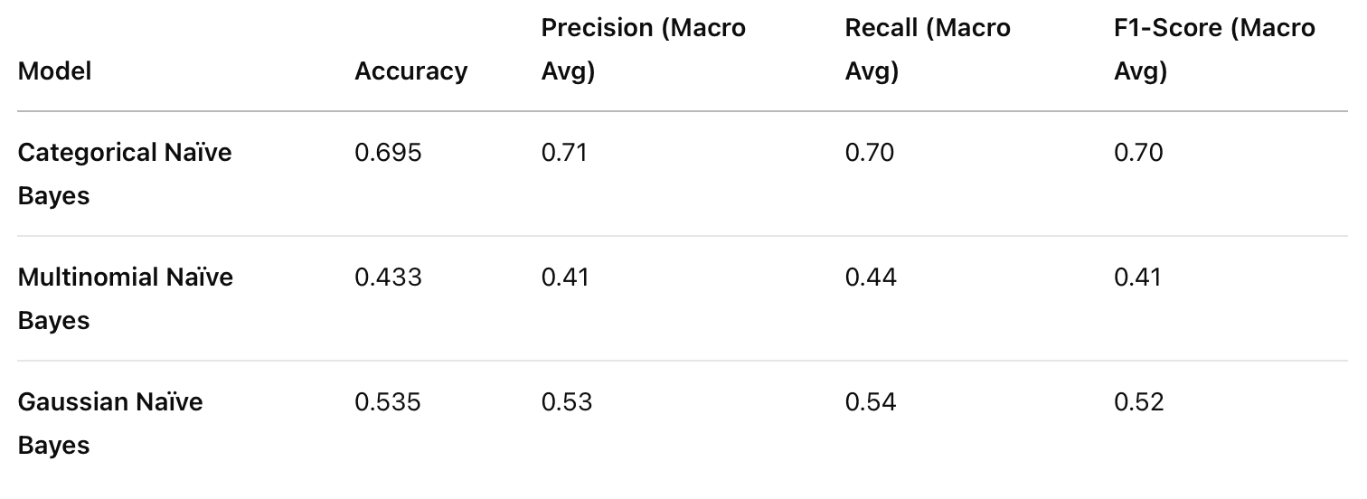
Comparison of all three NB models
Examining the three Naïve Bayes variants on the football player valuation dataset reveals distinct performance patterns:
- Categorical Naïve Bayes shows the highest overall accuracy (69.5%), making it the most effective model for this particular dataset. This suggests that categorical features like preferred foot, position, nationality, and club affiliation are strong predictors of a player’s market value.
- Gaussian Naïve Bayes achieved moderate performance (53.5% accuracy), indicating that numerical features such as age and performance metrics follow distributions that Gaussian NB can partially capture but with limitations.
- Multinomial Naïve Bayes performed poorest (43.3% accuracy), which is expected as this model is typically optimized for count-based features (like word frequencies) rather than the mixed feature types in this dataset.
Class-specific Performance
Looking at class-specific metrics reveals interesting patterns:
- Class 0 (Lower value players): All models perform relatively well at identifying this class, with Categorical NB showing high precision (0.84) and Gaussian NB showing high recall (0.81).
- Class 1 (Mid-value players): This appears to be the most challenging category to classify across all models, with Multinomial NB particularly struggling (precision: 0.30, recall: 0.16).
- Class 2 (High-value players): Categorical NB shows strong performance in identifying high-value players (recall: 0.81), suggesting categorical features strongly signal elite player status.
Connection to Dataset Features
The varying performance of these models highlights how different feature types contribute to player valuation:
- Categorical features (club, nationality, position) appear most influential in determining market value, as evidenced by Categorical NB’s superior performance. This aligns with football market realities where playing for prestigious clubs or being from certain countries often commands premium valuations.
- Numerical performance metrics contribute moderately to valuation predictions but may have complex relationships that aren’t perfectly captured by the Gaussian distribution assumption.
- The poor performance of Multinomial NB suggests that count-based approaches aren’t suitable for this data, indicating that absolute numbers (like total goals or appearances) may be less important than their context (position, club level, etc.).
Conclusion
Our analysis of three Naïve Bayes variants on football player data reveals that categorical features (club, nationality, position) are stronger predictors of market value than numerical performance metrics alone. This is evidenced by Categorical Naïve Bayes achieving the highest accuracy (69.5%) compared to Gaussian (53.5%) and Multinomial (43.3%) variants. Additionally, all models struggled most with classifying mid-value players, suggesting this category has less distinctive characteristics than low or high-value players.
These findings have important implications for football scouting and analytics departments. While performance statistics remain valuable, contextual factors like the prestige of a player’s club and their specialized position significantly influence market valuation. However, the moderate accuracy across all models indicates that player valuation is a complex task that likely requires more sophisticated modeling approaches to capture the non-linear relationships between player attributes and market value. Future work could explore ensemble methods or neural networks to improve predictive performance beyond what the Naïve Bayes family of algorithms can achieve.