
Football Analytics - Model Implementation - Logistic Regression
Overview
Linear regression is a statistical method that models the relationship between a dependent variable and one or more independent variables using a linear equation. It finds the best-fitting straight line through data points by minimizing the sum of squared differences between observed and predicted values. The resulting model estimates how the dependent variable changes when independent variables are varied.

Visual Respresentation of Linear Regression
Logistic regression is a statistical model used to predict binary outcomes by estimating the probability that an observation belongs to a certain category. It transforms linear predictions into probability values between 0 and 1 using a logistic function. Despite its name, logistic regression is a classification algorithm rather than a regression technique.
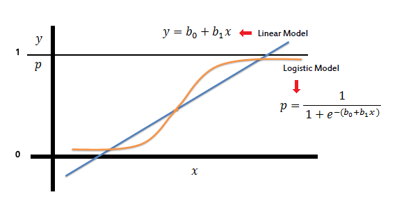
Visual Respresentation of Logistic Regression
Both methods use linear combinations of features for prediction and can be trained using optimization techniques. However, linear regression predicts continuous values and assumes a linear relationship between variables, while logistic regression predicts probabilities for categorical outcomes and models nonlinear decision boundaries.
Logistic regression uses the sigmoid function (also called the logistic function) to transform linear predictions into probability values between 0 and 1. The sigmoid function S(z) = 1/(1+e^(-z)) maps any real-valued number to a value between 0 and 1, creating the characteristic S-shaped curve that handles the classification threshold.

Visual Respresentation of Sigmoid Function
Maximum likelihood estimation is the method used to train logistic regression models by finding parameter values that maximize the probability of observing the given data. It works by formulating a likelihood function that measures how probable the observed data is under different parameter settings, then finding parameters that maximize this function. This approach helps logistic regression find optimal decision boundaries for classification tasks.
Logistic Regression Dataset
This dataset is similar to the dataset used for Multinomial Naive Bayes as we are doing a comparing here with the two models. We only filter out the target variable with class “2” so that the target variable becomes binary.
The dataset consists of football player attributes, including categorical and numerical features. These features help analyze how different factors influence a player’s market value.
Numerical Features:
- Performance Metrics Across Seasons: Includes appearances (MP), goals (G), assists (A), yellow cards (YC), red cards (RC), and other relevant statistics.
Target Variable:
- ValueCategory: Represents different categories of market value for a player, classifying them into three groups (0 or 1).
Data Preprocessing and Train-Test Split
Before training the model, several preprocessing steps are applied to ensure data quality and improve model performance:
-
Class Balancing: The dataset may have an imbalance in player value categories, meaning some categories may have significantly fewer samples than others. To address this, we perform resampling to ensure each class has an equal number of samples (1,000 per category).
-
Train-Test Split: The dataset is split into 80% training and 20% testing, ensuring that the model learns from a diverse set of data while being evaluated on unseen examples.
-
Outlier Handling: To prevent the model from encountering values in the test set that were not seen during training, any test set values exceeding the maximum observed training values in a particular feature are capped.
Screenshots and Links to Datasets
X-train

X-train for LR
The shape of X-train is (1600, 44). Link to dataset
X-test

X-test for LR
The shape of X-test is (400, 44). Link to dataset
y-train

y-train for LR
The shape of y-train is (1600,). Link to dataset
y-test
y-test for LR
The shape of y-test is (400,). Link to dataset
Code files
These files are used for the dataset preparation and model training can be found here
Results
Logistic Regression
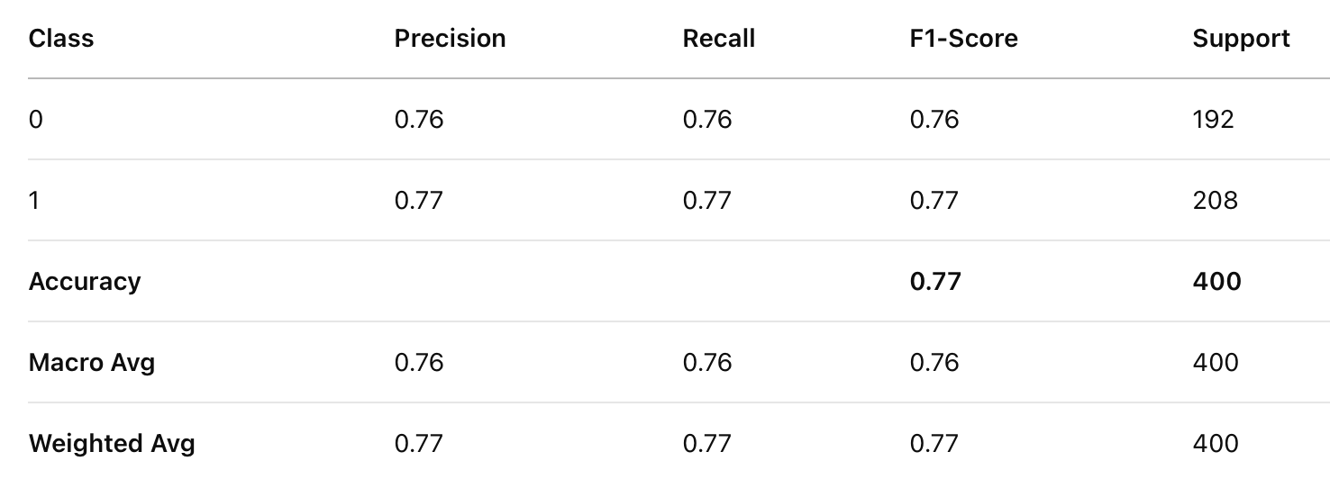
Classification Report for LR
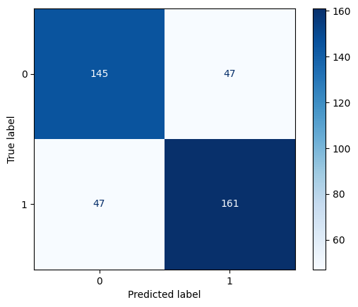
Confusion Matrix for LR
Multinomial Naïve Bayes
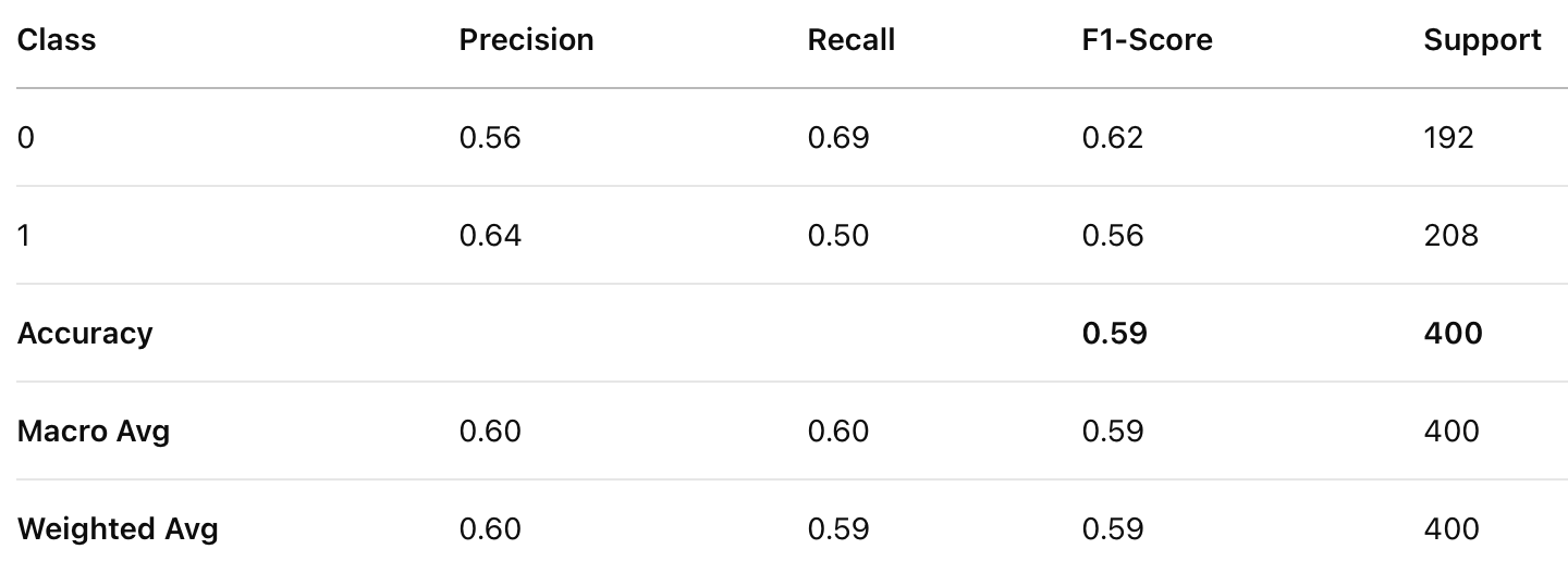
Classification Report for MNB
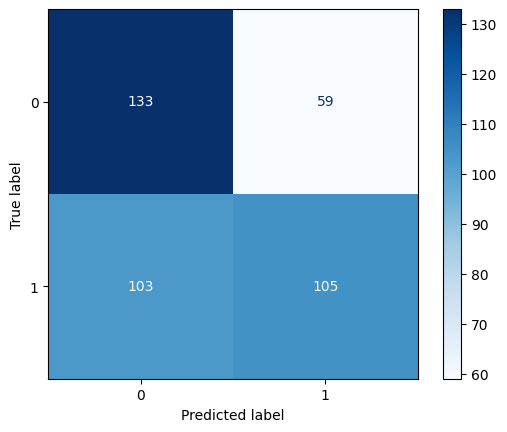
Confusion Matrix for MNB
Comparison of Models
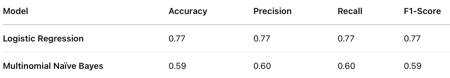
Comparison of Models
Logistic Regression significantly outperforms Multinomial Naïve Bayes in all evaluation metrics (Precision, Recall, and F1-score). Logistic Regression achieves an accuracy of 77%, whereas Multinomial Naïve Bayes reaches 59%, a substantial difference of 18%.
For class 0, Multinomial Naïve Bayes has higher recall (0.69 vs. 0.76 in Logistic Regression), meaning it correctly identifies more instances of class 0, but at the cost of lower precision (0.56 vs. 0.76). For class 1, Logistic Regression dominates in all metrics, with significantly better precision (0.77 vs. 0.64) and recall (0.77 vs. 0.50).
Conclusion
Logistic Regression generally handles numerical data better, while Multinomial Naïve Bayes is more suited for categorical or text-based data. Since the dataset contains numerical features (player performance metrics), Logistic Regression is a more natural fit.
Naïve Bayes assumes feature independence, which likely does not hold for this dataset. Many player attributes (e.g., goals, assists, and market value) are highly correlated. This assumption mismatch reduces Naïve Bayes’ effectiveness.
For this dataset, Logistic Regression is the superior model because it better captures the relationships between numerical performance metrics and the player’s market value category. Multinomial Naïve Bayes, which is more suitable for categorical data, struggles due to its independence assumption.