
Football Analytics - Model Implementation - Support Vector Machine
Overview
Support Vector Machines (SVMs) are one of the most powerful and versatile supervised learning models in machine learning, especially useful for classification tasks.
At their core, SVMs are linear classifiers — they aim to draw a hyperplane between classes in a dataset. But what makes SVMs truly powerful is their ability to handle non-linear data through a method called the kernel trick.
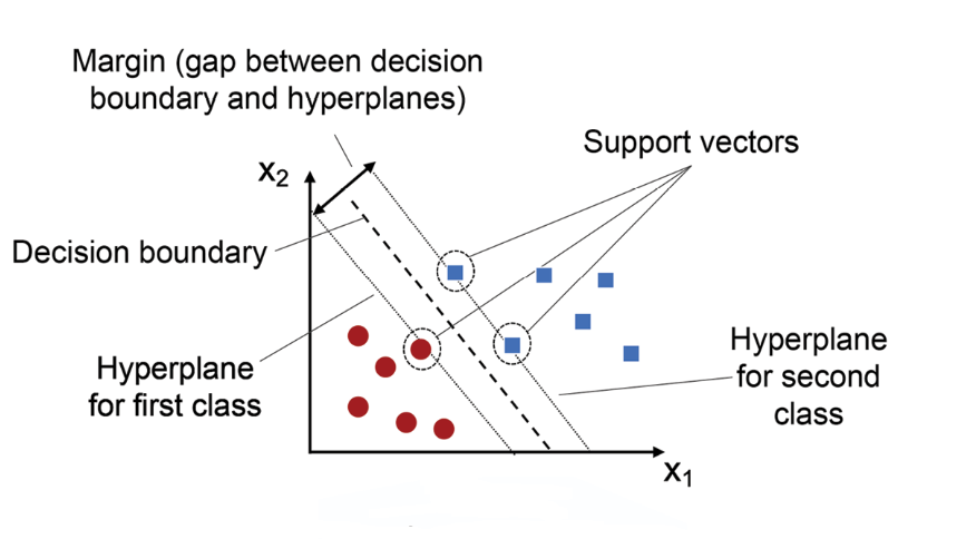
Visual Representation of SVM Classifier
How SVM Works
Imagine a dataset where two classes are neatly split by a straight line. This is the sweet spot for a linear SVM, which seeks to find the best separating line (or in higher dimensions, a hyperplane). SVMs look for the maximum margin separator — the hyperplane that is as far as possible from the nearest points of both classes, known as support vectors. This margin-based approach gives SVMs strong generalization abilities — they often perform well even on unseen data.
The Role of the Dot Product
SVMs make decisions based on the formula:
$f(x) = w^T \cdot x + b$ where:
- $w$ is the weight vector,
- $x$ is the input vector,
- $b$ is the bias term. The dot product $w^T \cdot x$ measures the similarity between the weight vector and the input vector. If the result is positive, the input belongs to one class; if negative, it belongs to the other.
Kernel Trick
The kernel trick is a powerful technique that allows SVMs to operate in high-dimensional spaces without explicitly transforming the data. Instead of computing the coordinates of the data in a higher-dimensional space, SVMs use kernel functions to compute the dot product directly in that space.
This is particularly useful for non-linear classification tasks. Common kernel functions include:
-
Linear Kernel: This is the simplest kernel, where the decision boundary is a straight line (or hyperplane in higher dimensions). It is defined as the dot product of two input vectors. Formula: $K(x_i, x_j) = x_i^T \cdot x_j$.
-
Polynomial Kernel: This kernel allows for non-linear decision boundaries by computing the polynomial of the dot product of two input vectors. Formula: $K(x_i, x_j) = (x_i^T \cdot x_j + r)^d$, where $r$ is a constant and $d$ is the degree of the polynomial.
-
Radial Basis Function (RBF) Kernel: This kernel is particularly effective for non-linear data. It computes the similarity between two input vectors based on their distance in the feature space. Formula: $K(x_i, x_j) = e^{-\gamma \left | \left | x_i - x_j \right |\right |^2}$, where $\gamma$ is a parameter that defines the width of the Gaussian kernel.
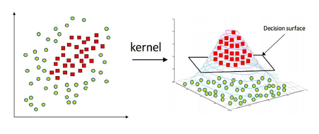
Visual Representation of Kernel Trick
Polynomial Kernel Example (r = 1, d = 2)
With $r=1$ and $d=2$, the polynomial kernel becomes:
$K(x_i, x_j) = (x_i^T \cdot x_j + r)^d$
To avoid confusion, let’s denote $x_i$ as $x$ and $x_j$ as $y$. The polynomial kernel can be expressed as:
$K(x, y) = (x^T \cdot y + 1)^2 = (\sum x_i y_i + 1)^2 = (x_{1}y_{1} + x_{2}y_{2} + 1)^2$
Expanding this expression gives us:
$K(x, y) = x_{1}^2y_{1}^2 + x_{2}^2y_{2}^2 + 2x_{1}y_{1}x_{2}y_{2} + 2x_{1}y_{1} + 2x_{2}y_{2} + 1$
The corresponding feature map is:
$ \phi(x_1, x_2) = (x_{1}^2, x_{2}^2, \sqrt{2}x_{1}x_{2}, \sqrt{2}x_{1}, \sqrt{2}x_{2}, 1)$
Now the original 2D point $(x_1, x_2)$ is mapped to 6-dimensional space.
Let’s say we have two points:
- Point A: $(1, 2)$
- Point B: $(3, 4)$
Let x = (1, 2) and y = (3, 4).
$\phi(1,2) = (1^2, 2^2, \sqrt{2} \cdot 1 \cdot 2, \sqrt{2} \cdot 1, \sqrt{2} \cdot 2, 1)$
$\phi(1,2) = (1, 4, 2\sqrt{2}, \sqrt{2}, 2\sqrt{2}, 1)$
$\phi(3,4) = (3^2, 4^2, \sqrt{2} \cdot 3 \cdot 4, \sqrt{2} \cdot 3, \sqrt{2} \cdot 4, 1)$
$\phi(3,4) = (9, 16, 12\sqrt{2}, 3\sqrt{2}, 4\sqrt{2}, 1)$
The polynomial kernel allows us to create a non-linear decision boundary in the original 2D space by mapping the data to a higher-dimensional space.
Advantages of SVM
- Effective in high-dimensional spaces (e.g., text classification, image recognition).
- Works well with small datasets where the number of features is greater than the number of samples.
- Robust to outliers (when using soft-margin SVM).
- Supports both linear and non-linear classification using kernel tricks.
Disadvantages of SVM
- Computationally expensive for large datasets.
- Sensitive to parameter tuning, especially C and kernel choice.
- Not easily interpretable, unlike decision trees.
- Struggles with overlapping classes, as it focuses on margin maximization.
Use Cases of SVM
Text classification (e.g., spam detection, sentiment analysis). Image recognition (e.g., face detection). Medical diagnosis (e.g., cancer classification). Bioinformatics (e.g., gene classification).
Dataset Preparation
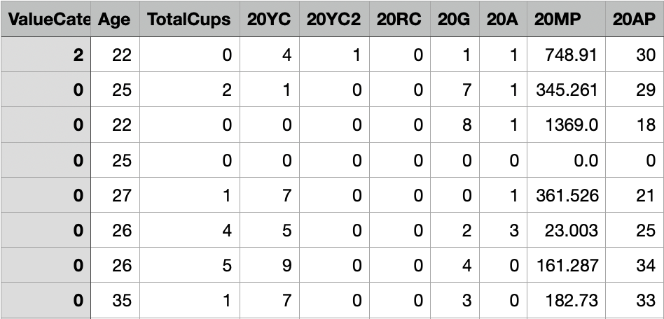
The dataset consists of football player attributes, including categorical and numerical features. These features help analyze how different factors influence a player’s market value.
Numerical Features:
- Performance Metrics Across Seasons: Includes appearances (MP), goals (G), assists (A), yellow cards (YC), red cards (RC), and other relevant statistics.
Target Variable:
- ValueCategory: Represents different categories of market value for a player, classifying them into three groups (0, 1 or 2).
Dataset before preprocessing:
Data Preprocessing and Train-Test Split
Before training the model, several preprocessing steps are applied to ensure data quality and improve model performance:
-
Class Balancing: The dataset may have an imbalance in player value categories, meaning some categories may have significantly fewer samples than others. To address this, we perform resampling to ensure each class has an equal number of samples (1,000 per category).
-
Train-Test Split: The dataset is split into 80% training and 20% testing, ensuring that the model learns from a diverse set of data while being evaluated on unseen examples.
-
Outlier Handling: To prevent the model from encountering values in the test set that were not seen during training, any test set values exceeding the maximum observed training values in a particular feature are capped.
-
Standardization: The numerical features are standardized to have a mean of 0 and a standard deviation of 1. This step is crucial for SVMs, as they are sensitive to the scale of the input features.
The train test split random seed is the same for all models to ensure consistency in the results.
Screenshots and Links to Datasets
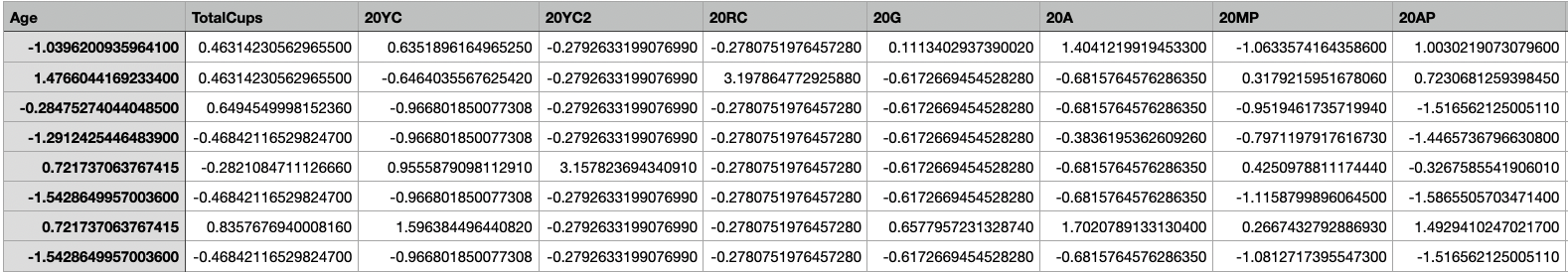
X-train
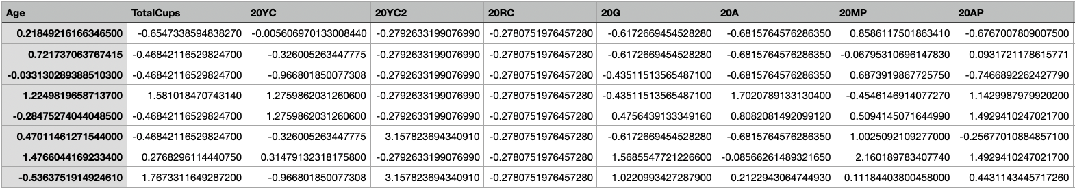
X-train for SVM
The shape of X-train is (1600, 44). Link to dataset
y-train
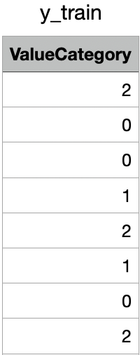
y-train for SVM
The shape of y-train is (1600,). Link to dataset
X-test
X-test for SVM
The shape of X-test is (400, 44). Link to dataset
y-test
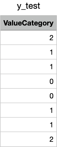
y-test for SVM
The shape of y-test is (400,). Link to dataset
Code files
The code used for dataset preparation and training the Support Vector Machine models is available here
Results
We perform experiments with kernels such as Linear, Polynomial, and RBF. We also test it out with different values of C (0.1, 1, and 10) to see how it affects the model’s performance. The decision boundary is visualized using PCA to reduce the dimensionality of the data to 2D.
Linear Kernel
C = 0.1
Classification Report for Linear Kernel SVM with C=0.1
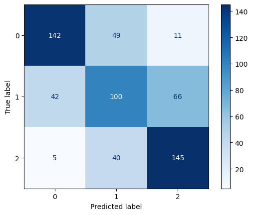
Confusion Matrix for Linear Kernel SVM with C=0.1
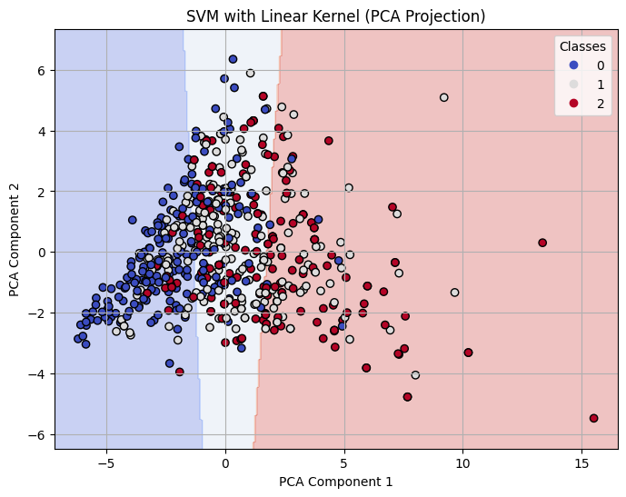
Decision Boundary on 2-D PCA for Linear Kernel SVM with C=0.1
C = 1

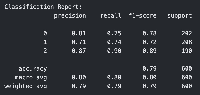
Classification Report for Linear Kernel SVM with C=1
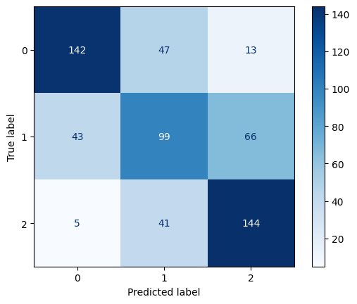
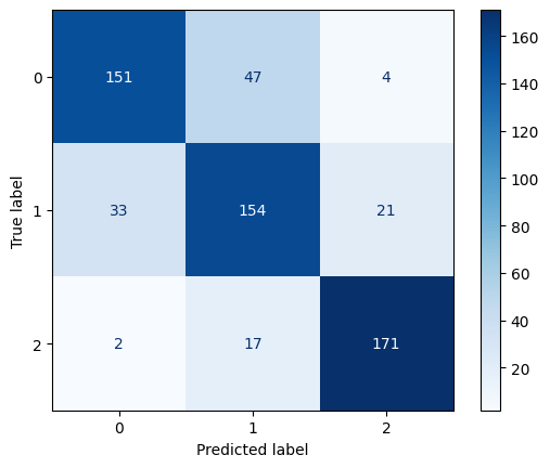
Confusion Matrix for Linear Kernel SVM with C=1
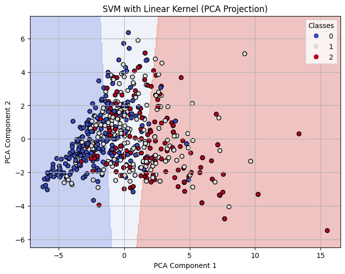
Decision Boundary on 2-D PCA for Linear Kernel SVM with C=1
C = 10
Classification Report for Linear Kernel SVM with C=10
Confusion Matrix for Linear Kernel SVM with C=10

Decision Boundary on 2-D PCA for Linear Kernel SVM with C=10
RBF Kernel
C = 0.1
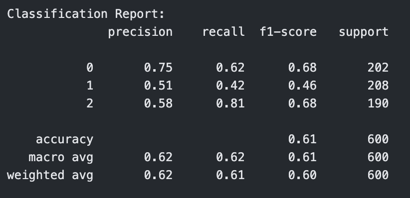
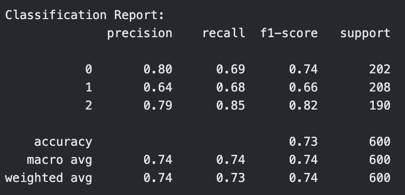
Classification Report for RBF Kernel SVM with C=0.1
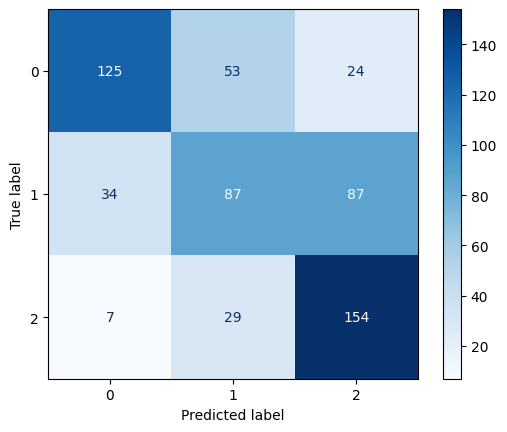
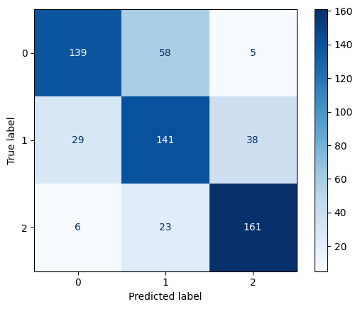
Confusion Matrix for RBF Kernel SVM with C=0.1
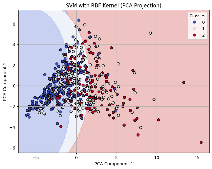
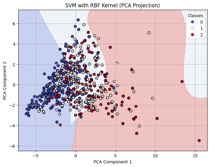
Decision Boundary on 2-D PCA for RBF Kernel SVM with C=0.1
C = 1
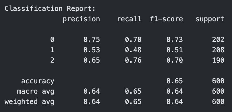
Classification Report for RBF Kernel SVM with C=1
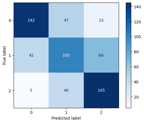
Confusion Matrix for RBF Kernel SVM with C=1
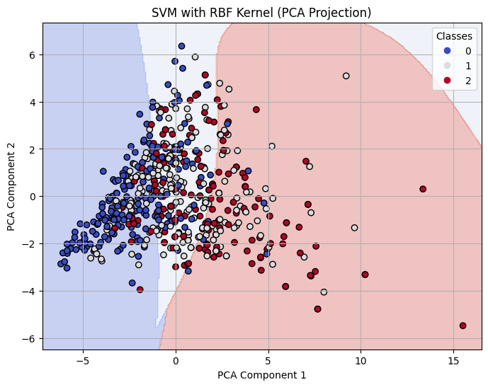
Decision Boundary on 2-D PCA for RBF Kernel SVM with C=1
C = 10
Classification Report for RBF Kernel SVM with C=10
Confusion Matrix for RBF Kernel SVM with C=10
Decision Boundary on 2-D PCA for RBF Kernel SVM with C=10
Polynomial Kernel
C = 0.1
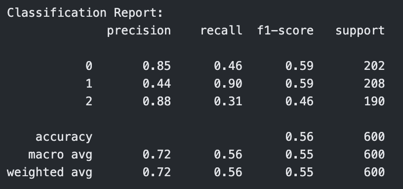
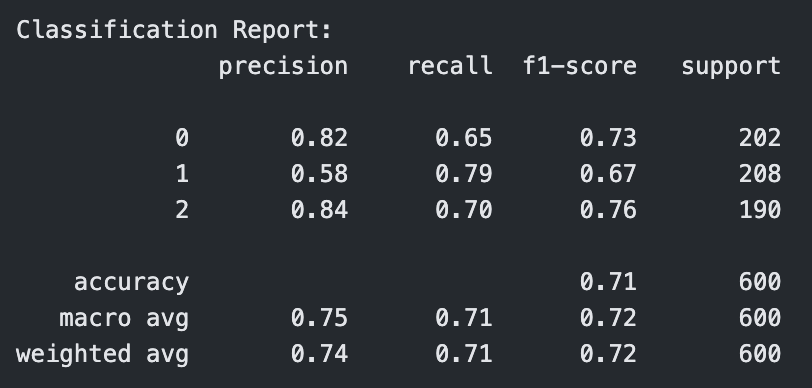
Classification Report for Polynomial Kernel SVM with C=0.1
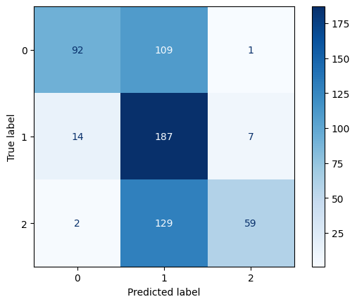
Confusion Matrix for Polynomial Kernel SVM with C=0.1
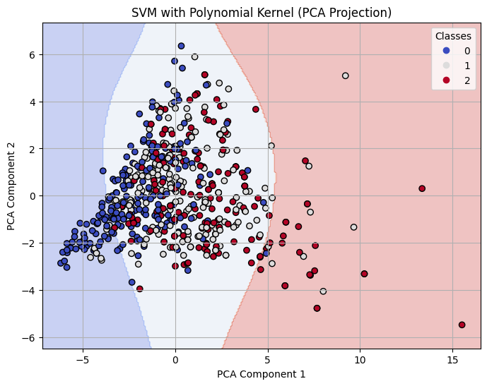
Decision Boundary on 2-D PCA for Polynomial Kernel SVM with C=0.1
C = 1
Classification Report for Polynomial Kernel SVM with C=1
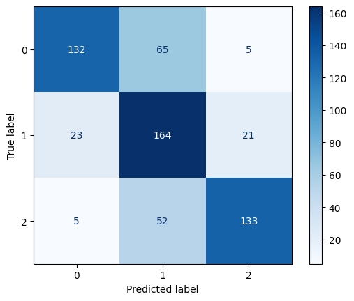
Confusion Matrix for Polynomial Kernel SVM with C=1
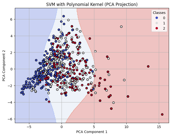
Decision Boundary on 2-D PCA for Polynomial Kernel SVM with C=1
C = 10
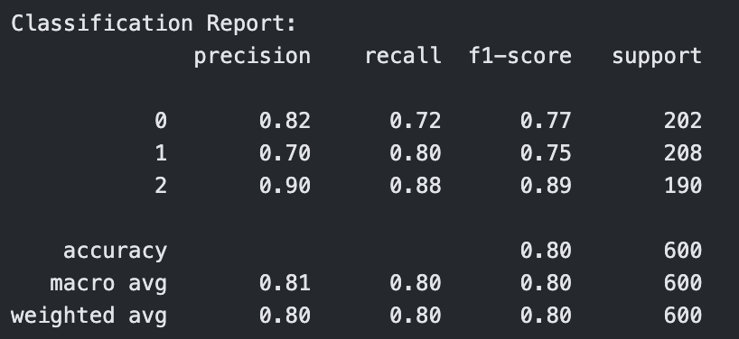
Classification Report for Polynomial Kernel SVM with C=10
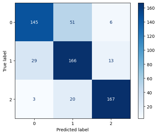
Confusion Matrix for Polynomial Kernel SVM with C=10
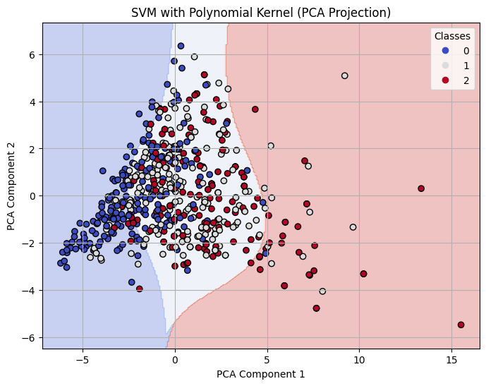
Decision Boundary on 2-D PCA for Polynomial Kernel SVM with C=10
Comparison of Models
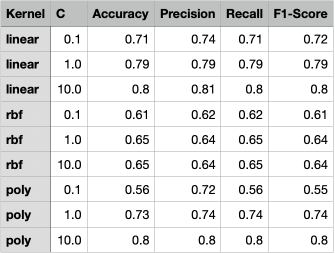
Comparison of SVM Models
For both linear and polynomial kernels, accuracy increased as C increased. The RBF kernel, however, did not show significant improvement with higher C values. For RBF, the accuracy gain had stopped after C = 1, indicating that the model was not learning effectively from the data.
Linear Kernel
The linear kernel showed steadily improving performance as the cost parameter increased. At C = 0.1, the model had moderate accuracy (0.71), but when increased to C = 1, the model improved significantly across all metrics, reaching 0.79 in accuracy, precision, recall, and F1-score. At C = 10, it performed the best among linear models, achieving an accuracy of 0.80 and an F1-score of 0.80, indicating strong generalization with minimal overfitting.
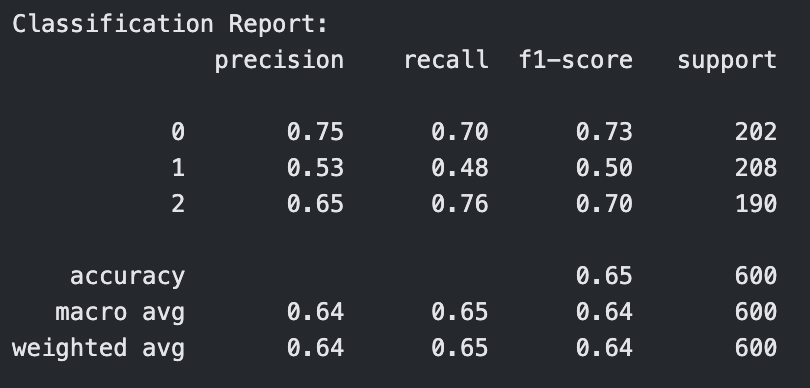
RBF Kernel
The RBF kernel underperformed relative to the other kernels, especially at C = 0.1, where it had an accuracy of 0.61. Even at C = 1 and C = 10, the performance plateaued around 0.65 accuracy and F1-score, showing that the model struggled to find effective nonlinear boundaries for the given data. This suggests that the RBF kernel may not be well-suited to this dataset or requires more extensive hyperparameter tuning (e.g., gamma).
Polynomial Kernel (Degree 3)
The polynomial kernel with degree 3 showed mixed results. At C = 0.1, it performed the worst across all models with an accuracy of 0.56 and F1-score of 0.55. However, as C increased, its performance improved significantly. At C = 1, it reached an accuracy of 0.73, and at C = 10, it tied with the best linear model with an accuracy and F1-score of 0.80. This indicates that higher capacity polynomial models can be effective with the right regularization.
Conclusion
The best performing model overall is the SVM with either a linear kernel or a polynomial kernel (degree 3) and C = 10, both achieving an accuracy of 80%. However, between the two, the linear kernel model is preferred due to its simpler structure, which generally leads to faster training, better interpretability, and lower risk of overfitting compared to higher-degree polynomial kernels.